Genetic Algorithms to Solve the Motion Planning Problem

Abstract: Motion planning is a field of growing importance as more and more computer controlled devices are being used. Many different approaches exist to motion planning|none of them ideal in all situations. This paper considers how to convert a general motion planning problem into one of global optimisation. We regard the general problem as being the classical configuration space findpath problem, but assume that the configurations of the device can be bounded by a hierarchy of hyper-spheres rather than being explicitly computed. A program to solve this problem has been written employing Genetic Algorithms. This paper describes how this was done, and some preliminary results of using it.

Key Words: Motion Planning, Path Optimisation, Complex Geometries

Category: G.1.6, I.2.8, I.2.9, I.2.10

1 Introduction

Motion planning is the algorithmic calculation of a set of movements for one or more controllable objects. This motion aims to achieve a certain goal, while not violating any of the given restrictions. Common examples of this problem include that of moving a robot vehicle between two given positions and orientations, or moving a robot arm between a start and goal poise. These examples are both cases of the classical motion planning problem called findpath, in which the only other constraint on motion is that it be collision-free; more complex variations of the general motion planning problem might also include (say) velocity constraints. In many motion planning problems, there are several possible solutions; depending upon the circumstances, one may be better than another. On what grounds the choice is made depends greatly upon the final use of the plan. Minimising the planning time (ie. finding the first feasible solution) is common, as is minimising the time for the motion (ie. getting the vehicle from start to finish as fast as possible).

A motion-planning algorithm needs to be constantly "aware" of where all parts of the vehicle (or whatever is being moved) are. For example in a car, it is no good ensuring that the driver's side front corner makes it through the gate if the passenger's side mirror gets broken off. Of course the problem is compounded if the vehicle isn't a rigid body (eg. a trailer is being towed behind). This constant testing of all parts of the vehicle against near-by obstacles becomes very computationally expensive|especially with more complicated vehicles or environments.

Although motion planning problems can be devised for a wide range of mechanical devices (not just robots), a mathematical concept called configuration space can be used to make the problems look more alike. For a given device we look at its number of degrees of freedom (dof), and assign configuration variables (say, p₁ , p₂ , . . . ) to each way that the device can move. So, for example, a robot vehicle might be assigned variables to describe its position and orientation, whereas an industrial robot arm with 5 rotary joints might be described by . Each of the n independent configuration parameters can then be assigned a coordinate axis in an n-dimensional configuration space, and the motion planning problem restated as finding a line in that space joining the start and goal configurations [Lozano-P erez, 1983]. Obstacles in real space then map to obstacles in the configuration space (i.e., configuration space obstacles or CSOs), which are simply the configurations that would cause the device to collide with the obstacle (in real space) or are otherwise illegal (eg. joint out of range).

In theory then, a solution to the findpath problem for general configuration spaces will act as a solution to the findpath problem for any device. In practise, reality is not nearly as simple for a number of reasons. Firstly, we need to be able to describe the CSOs, and even for simple shapes these may map into complex, high-dimensional structures in configuration space. For example, polyhedra commonly map into polytopes with helical surfaces. Secondly, even if a solution is found for the findpath problem, physical constraints (such as the accuracy to which we can move the device) may still determine whether that path is useful. Finally, the time taken to search configuration space for a solution is often very large. But if we bear these problems in mind configuration space is still a useful tool [Latombe, 1991].

Here we show how a genetic algorithm [Goldberg, 1989] can be used to solve the general findpath problem. Our genome encodes an entire path from start to goal configuration; this path may well not be feasible, although clearly only those final genomes that are feasible are of interest. Noting the problem of computing the CSOs mentioned above we instead assume that the CSOs can be approximated by a hierarchical data-structure called a sphere tree; this structure can be generated from CAD data for the original objects, together with standard bounds on the device motion. To prove the concept we have implemented the algorithm for the general case, and present some results in this paper.

2 Problem Definition

As mentioned earlier, there are many different classes of motion planning problems, and different strategies work better in some cases than others. The particular class considered in this paper has n-dimensional configuration space with spherical (possibly overlapping) obstacles. The environment is taken to be bounded by a n-dimensional hyper-cube of side 1. The path to be found between the given start and finish points is piecewise linear with a (given) fixed number of segments. This representation allows easy testing of whether a particular path is contained within free-space or not. The planning algorithm is assumed to have complete and accurate knowledge of the environment.

There exist a number of algorithms which form an approximate decomposition of an obstacle of any shape into a hierarchy of shape descriptions, with fi each level of the hierarchy describing the shape as a set of overlapping spheres [del Pobil and Serna, 1995, Pitt-Francis and Featherstone, 1998]. It is possible to construct sphere hierarchies for the CSOs to any desired degree of accuracy [Featherstone, 1995]. Thus in this paper we assume such a set of (hyper-) spheres is available to describe the CSOs. Not only is this description generally available, but calculating the interactions between the path and spheres is generally far simpler than between paths and the original complex obstacle|especially if the device to be moved has joints, allowing many degrees of freedom. The imposition of a unit hyper-cube as the boundary is not limiting either: the different dimensions of the original problem can be scaled as necessary, and non-rectangular boundaries can be achieved by adding virtual obstacles to the configuration space.

So the program is given: the dimension of the space n; the start and finish positions S, F; the number of segments m; and a set of obstacle centres O₁, ..., O_p and radii r₀, ... , r_p . Any particular path stretches from the start to the finish, going through m - 1 intermediate points; and so is completely represented by those m - 1 points. The planning problem is solved when a set of such points is found which defines a path that intersects with none of the spheres.

3 Re-formulation as an GA

Given the above description of the problem, what is required is to transform this into an optimisation form that may be amenable to a quick solution. This has been done, and the details of how a genetic algorithm has been used follow a brief discussion of previous related work. While several optimisation strategies are possible (GAs being only one of these), it is necessary for it to be one that finds global optima.

3.1 Overview of GAs

Genetic algorithms[Goldberg, 1989] are part of a class of what is known as Evolutionary algorithms. Evolutionary algorithms are computational models that solve a given problem by maintaining a changing population of individuals, each with is own level of fitness. The change in the population is achieved by the selection, reproduction and mutation procedures within the method. The operation of these three procedures is dependent upon the fitness of the individuals concerned.

Genetic algorithms are characterised by the fact that all the information for any individual in the population is encoded using some linear encoding system, This (usually binary) encoding is intended to be analogous to natural DNA.

Cross-over is the means by which two different genomes (ie. members of the population) can combine to form a new genome. One such method for this is known as uniform cross-over. It works by creating a random bit mask of the same length as the genomes. The new gene is formed by taking the value from the nth position of the first gene if the nth value of the mask is a 1, otherwise taking the value of the nth position in the second gene.

Selection is where it is decided which members of the population will be preserved, and which will be replaced. It is usually done via a weighted random selection|the weighting is based upon the fitness of the individual. That is, the

more fit members of the population have a greater chance of progressing to the next generation. The same method is used to select pairs of parents which will, using the cross-over methods described above, give the replacements.

Each newly created individual is subject to mutation. Each bit within these individuals is, with a very small probability, inverted. It may be that certain genes required for a correct solution are not present in any of the initial random population. Mutation then, is a means of introducing genetic diversity into the population.

3.2 Related work

This is not the first time that researchers have attempted to apply genetic algorithms to solve motion planning problems. [Han et al., 1997] give a motion planning algorithm for two dimensional problems.

They in fact describe the algorithm as a dynamic one (ie. one that supports moving obstacles) but this is a little misleading. The method described for achieving this is to simply re-run the algorithm at intervals throughout the motion, to create new paths based upon the new obstacle positions. A similar means of attaining dynamic motion planning is employed in [Talbi et al., 1992]. The encoding employed means that the path must monotonically approach the goal. With this restriction, the algorithm will be unable to find a solution in many environments with overlapping obstacles even though there is one. Unlike the algorithm proposed here, [Han et al., 1997]'s algorithm does make some attempt at optimising the path|it attempts to find a path as close as possible to the trivial straight-line solution.

[Toogood et al., 1995] have designed a planner to solve the specific case of manipulators with three rotating joints. Again, the path (in real space) must monotonically approach the the goal. The algorithm can be directed to prefer optimal paths, for varying definitions of optimal (eg. minimising distance or minimising maximum torque required).

[Bessiereand et al., 1993] is a little different. It is uses genetic algorithms in the sub-planner of a larger non-GA based algorithm. Also, the encoding is not chosen so that that the path always connects the given start and goal points, but instead simply extends from the start. It is then the goal of the fitness function to ensure that the path meets the end (as well as avoiding obstacles). The reason for this is that the encoding is not coordinate based (as the previous cited works, and this paper use). Instead, the path encoding (or to be more accurate, the sub-path encoding since the genetic algorithms are only employed in the sub-planner) consists of a series of sequential Manhattan moves (ie. a piecewise linear path, with all segments parallel to one of the coordinate axes).

3.3 Encoding

Each member of the population is a single, complete, m-segment path joining the start to the finish. This path can be described in m - 1 points, each of n dimensions, and so by a total of mn oating point values, each within [0, 1]. These oating point values can be approximated by the integers [0,Max] (eg. if Max = 65535, then = 8060 and therefore 0.123 8060/65535 and so 0.123 is represented by the integer 8060). Finally, if Max is chosen to be

one less than a power of 2 (ie. Max = 2^b - 1), then the entire path can encoded as a nmb long string of bits. By choosing this representation, any random nmb long string of bits corresponds to a valid path from the start to the finish, entirely contained within the unit hyper-cube.

3.4 Evaluation

Two different evaluation functions have been implemented and are discussed. The first of these is straight-forward: given any path, the function simply returns an integer which is the number of distinct obstacles that the input path crosses. A geometric calculation yields this easily.

For each combination of sphere and path segment in turn: a line is constructed which passes through, and is perpendicular to, the line in which the segment lies. It is also constrained to pass through the sphere's centre. If the point at which these two lines intersect lies outside of the path segment, then the critical length is taken to be the smaller of the two distances from the segment's ends to the sphere's centre.

If the point where the lines intersect lies within the segment, then the critical length is the distance from that point of intersection to the sphere's centre. The line and sphere intersect if and only if the critical length is smaller than the radius of the sphere.

Repeating this for all possible combinations of spheres and path segments and summing up yields the required value. This has an obvious minimum of zero, occurring when all segments of the path are clear of obstacles. If such a path is ever found, then the algorithm may terminate returning this as a complete, valid and collision-free path.

While being relatively simple (both in conception and implementation), it does have the result that many changes in the path do not give rise to corresponding changes in the path's evaluation (ie. changes in the path can be quite significant, but if it still crosses the same set of obstacles, then it still receives the same scoring). The solution to this, is to treat each intersection not as a boolean value, but rather as a oating point value indicating how close to the tangential (non-crossing) position the line is. Segments that don't cross spheres score zero, but those which do cross, score a positive value proportional to the extent of the penetration. The desired path is one which crosses no obstacles, and so scores zero|again giving a definite target for any minimisation strategy.

It is worthy of note that in both these versions, the geometrical details are carefully abstracted away from the optimisation algorithm. The optimisation module deals with the paths only as black boxes whose interface allows them to be manipulated via bit-strings. When evaluation of the fitness function is required, then a simple eval() routine is called and a hidden implementation containing all the geometric aspects and calculations is executed. This separation helps keep the algorithm clean, and allows for the environment's and path's representation and the evaluation function to be changed without effecting the optimisation module.

Thus although we promote the use of the sphere hierarchy here, the genetic algorithm could in theory be used with other representations of CSOs.

3.5 Selection and Crossover

In each generation, one half of the population is replaced by new paths formed from the union of two others. Uniform random crossover is used. To select paths to be replaced, a biased random choice is made; the probability of a path being chosen for replacement is linearly proportional to its score. No path is replaced twice in one generation. The selection of parents is also done by biased random selection. The probability of path p_i, with score s_i, being chosen is linearly proportional to: max_j (sj ) + 1 - s_i .

One of the paths replaced may be a parent before its replacement, but no new path is a parent in the generation it is created. Each new path has two distinct parents, neither of which was its predecessor.

3.6 Mutation

Mutation is performed only on newly generated paths. Approximately MuteRate ( [0,1]) of paths are selected. If selected for mutation, then a single randomly chosen bit in that path's representation is reversed.

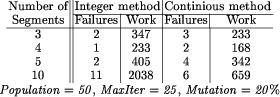
3.7 Post-processing

If the number of segments specified is greater than is actually required to find a feasible path, then it often happens that the resultant path can be pruned to remove unnecessary points. In addition, the path may involve turns which are sharper than required or approaches to obstacles which are closer than required (both of these can be a source of problems if the resultant path is to be executed by a mechanically controlled robot). Various means exist to post-process the feasible paths into more optimal (for varying definitions of optimal), but this goes beyond the scope of this paper.

4 Results

An n-dimensional program based upon the above algorithm has been implemented in C++ and tested on several platforms.

The results tabulated and discussed here were all performed in two dimensions for ease of verifying that solutions to the randomly generated problems do exist. In each case twenty feasible random problems were generated, each containing ten randomly sized and located circular obstacles. All the tables below show pairs of numbers. The first of these is the number times (out of the twenty runs) that the program failed to find a feasible solution in less than MaxIter iterations. The second is an indication of the average amount of work (the number of paths checked for obstacle intersections) required to obtain a solution. This average was obtained by taking the total amount of work done in the twenty trials, and dividing it by the success rate.

[Table 1] shows an interesting point of motion planning: namely that for problems of this type with a given complexity (in this case 10 obstacles), then there is usually an optimum number of segments. Choosing too few obviously makes the problem insolvable as there is not enough exibility permitted in the solution path for all obstacles to be avoided. In the opposite case, providing

too much exibility makes the task more difficult, as now more segments must be arranged to be clear of obstacles. The data in this table exhibits this quite clearly: the optimum for this set of problems is around 4. The increase in work for the higher value of 10 is quite marked.

The other important aspect indicated by this table is the difference that the choice of evaluation strategies makes. The results in columns two and three were obtained employing the first of the evaluation strategies discussed, where the (integer) number of obstacle crossings is used. Columns four and five instead used the continuously defined function that indicates the extent of the crossing. This continuous method, clearly requires less work to achieve a result. This was expected, as the continuous evaluation function does give the algorithm more information to work with. In particular, it gives an indication of whether a small movement in the path (which may still be crossing the same number of obstacles) is an improvement or not.

The table shows the improvement this extra information provides in all of the values, but it is particularly apparent in more complex problems. It is anticipated that such improvements will continue with further increases in the complexity.

In [Table 2] and [Table 3], results shown are produced using the integer evaluation method.

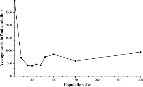
[Table 2] shows the effect of varying the population size on the efficiency and efficacy of the algorithm. To keep the comparisons fair, then the upper limit on the amount of work that each algorithm was permitted per run was kept a constant. That is, MaxIter x Population = 1250 . This allows the failures to be easily compared, as the maximum number of path evaluations allowed was the same. It is quite evident from the average work values that too low a population (not allowing sufficient genetic diversity) or too large a population (preventing sufficient iterations from being done) results in a significant performance loss. These figures have been plotted an appear in [Figure 1]. This shows that an optimal population for this particular problem exists, and is around 50.

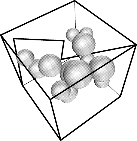
[Table 3] shows the effect of changing the mutation rate (the percentage of new paths which are mutated). Small populations (such as used here) tend to be prone to low genetic diversity, and so suffer a slowing of convergence. In these cases, some mutation is definitely beneficial. However too high a level of mutation destroys the good properties of the new paths before they can propagate. The detrimental effects of very high mutation can be seen from the results.

[Figure 2] shows the sample output of the program when run in three dimensions with 15 randomly placed spherical obstacles. The program sought to find a path from the lower left hand corner, to the upper right. A four segment path found by the program that satisfies this is shown.

5 Conclusions and Future Directions

We have presented here, a novel way of applying genetic algorithms to the field of motion planning. This was achieved by transforming a motion planning problem into a global optimisation one|the kind of problem for which genetic algorithms are particularly suited. A program has been implemented and the results of running this on some two-dimensional problems has been discussed.

One possibility that has not yet been explored in this paper is to seek not just a feasible path, but an optimal one. Of course what precisely \optimal" is varies upon what the path is to be used for. A common goal is to minimise total path distance. This could be achieved by changing the evaluation function to be C.Crossings + Length. The constant C would have to be made sufficiently large that an unnecessary crossing is never performed to save distance. Such an alteration is likely to slow down the convergence significantly, but in our experience such optimal solutions to the motion planning problem are only required

for motions that will be repeated many times, and for which the extra effort of minimising the cost is worthwhile. There is also a problem in confirming that the so-called \optimal solution" is optimal; however as the general motion planning problem is known to be exponential in its time complexity this diffculty should not surprise us [Canny, 1988].

Alternatively, the minimum clearance from any obstacle could be maximised. This is very desirable for a path if there is the possibility of inaccuracy in the motion of the robot that executes the resultant path. In this instance, the function is simpler, merely MinClearance. Note that a path that crosses any obstacle will have a negative minimum clearance, and so a correspondingly large evaluation, thus making the Crossings component redundant.

Rather than using a fixed sphere heirarchy, it should be possible to start: with a relatively coarse (but small) set of spheres; find a motion plan for that; and then refine the plan by using progressively finer collections of spheres from the hierarchy. Further work is required on this, and also on experiments to higher dimensional configuration spaces. Given the generality of the approach described, this is mainly an issue of implementing the algorithms for generating the CSOs from [Featherstone, 1995].

In all, we have shown that this new algorithm works well for the cases tried so far. We believe that it has potential to work on more complex problems, and in particular problems with more degrees of freedom.

References

[Bessiereand et al., 1993] Bessiereand, P., Ahuactzinand, J.-M., Talbi, E.-G., and Mazer, E. (1993). The ariadne's clew algorithm: Global planning with local methods. In Proceedings of the IEEE International Conference on Intelligent Robots and Systems, pages 13731380, Yokohama, Japan.

[Canny, 1988] Canny, J. F. (1988). The Complexity of Robot Motion Planning. MIT Press, Cambridge.

[del Pobil and Serna, 1995] del Pobil, A. P. and Serna, M. A. (1995). Spatial representation and motion planning. Springer-Verlag, Berlin/Heidelberg/New York.

[Featherstone, 1995] Featherstone, R. (1995). A hierarchical representation of the space occupancy of a robot mechanism. In Workshop on Computational Kinematics, Sophia-Antipolis, France. INRIA.

[Goldberg, 1989] Goldberg, D. (1989). Genetic algorithms in search, optimization, and machine learning. Addison-Wesley.

[Han et al., 1997] Han, W.-G., Baek, S.-M., and Kuc, T.-Y. (1997). Genetic algorithm

based path planning and dynamic obstacle avoidance of mobile robots. In Proceedings of the IEEE International Conference on Systems, Man and Cybernetics, volume 3, pages 2747-2751, Orlando, FL, USA.

[Latombe, 1991] Latombe, J.-C. (1991). Robot Motion Planning. Kluwer Academic Publishers.

[Lozano-Pérez, 1983] Lozano-Pérez, T. (1983). Spatial planning|a configuration space approach. IEEE Transactions on Computers, C-32(2):108-120.

[Pitt-Francis and Featherstone, 1998] Pitt-Francis, J. and Featherstone, R. (1998). Automatic generation of sphere hierarchies from cad data. In IEEE Int. Conf. Robotics & Automation, pages 324-329, Leuven.

[Talbi et al., 1992] Talbi, E.-G., Besiere, P., Ahuactzin, J.-M., and Mazer, E. (1992). Parallel robot motion planning in a dynamic environment. In Proceedings of the Second Joint International Conference on Vector and Parallel Processing, pages 835-836, Lyon, France. Springer-Verlag.

[Toogood et al., 1995] Toogood, R., Hao, H., and Wong, C. (1995). Robot path planning using genetic algorithms. In Proceedings of the International Conference on Systems, Man and Cybernetics, volume 1, pages 489-494, Vancouver, BC, Canada. IEEE.