Mental Models to Represent Dynamics - Using the Example "factorial"

Abstract: To use hypertext/hypermedia elements in teaching at universities an author not only needs knowledge of the technological possibilities. In addition he/she has to renew a here so called mental model of the relevant aspects of the material to be transferred. For the author, this last mentioned problem seems to be a central and often very complicated and time consuming one.

Key Words: Mental model, presentation of dynamics, animation

Categories: H.5.1, H.5.4

1 Introduction

The technical developments in recent years very often suggest to present lectures "out of the computer". Many progressive lecturers develop presentations of talks and/or lectures using presentation programs like e.g. PowerPoint. Especially presentations of dynamics will become possible thanks to the new technical features such as the generation of animations as well as videos.

In order to present elements of dynamics an author naturally needs to know how to generate these elements. But in my opinion in addition to the technical possibilities it is essential to generate an adequate mental model appropriate for the given presentation. This task which is associated to the usage of these new possibilities seems to me to be central . It requires deep insights into the material to be presented and thus is not to delegate to the staff responsible for the technical generation of the material. In my opinion many lecturers who are not familiar with these techniques totally oversee or at least strongly underestimate this problem.

In this contribution the mentioned problem of developing adequate mental models will be clarified by looking at the problem of introducing recursion with an example, namely factorial(3). Starting with a representation as can be found in the book [DoberDiss 96] the mental model has to be enhanced/refined such that all relevant steps can be shown explicitly. This leads to an animation of this example that can be found in [Dittrich 01]. Alternatives will be mentioned.

2 A Mental Model for the Example "factorial"

We will give an introduction into the handling of recursion in programming languages using the example of factorial formulated recursively (here in C++). Therefore we have to model all relevant aspects of function invocations explicitly. In my opinion, the analysis of this problem leads to the explicit representation of the following aspects:

• code of the function and its application in a program (1)
• implications of (repeated) function invocations
• generation and stacking of function invocations (2)
• generation and stacking of internal environments (3)
• output of the execution of the program (4)
• comment on the actual situations and of the transitions between them.(5)

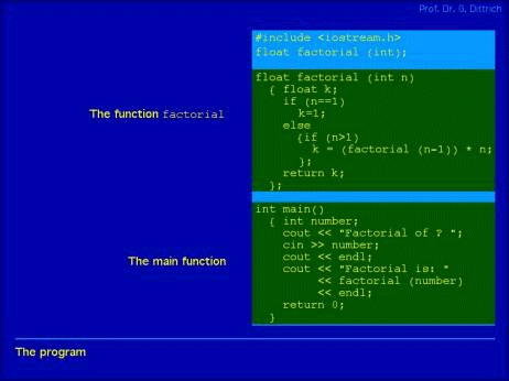
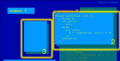
This is a very rough and still to be refined description of the mental model. In this case study they appear in a natural manner and will be shown later in our animation. These aspects should be represented in the right order as complete as possible though comprehensible at every point in time. Last but not least the presentation has to be completely reproducible and to be learned with individually adapted velocity.

3 Technical Conversions into Presentations

In a book (cf. e.g. [DoberDiss 96]) usually the running of a program is described in textual form, eventually enhanced by graphics including a set of different overlaid snapshots.

This representation requires the reader to generate his own comprehensive model in his head, where to reproduce the running of the program along the given description and the graphics. If one is in the situation to start to learn these phenomena, this sort of representation proves to be very rudimentary and thus often not easy to understand.

A good teacher/lecturer is much better in transferring insights into e.g. recursive invocations, when he/she applies traditional means for representations on a blackboard. Appropriate representations of internal situations include concrete values of relevant variables which can be wiped off and replaced by new values according to the different steps defined in the program. . An alternative is to apply transparencies even with overlays.

But this representation usually includes some drawbacks as well. On the one hand usually only a part of the entire situation will be represented explicitly (e.g. one has to have in mind the code and the place, where and in which invocation the program is actually running). On the other hand when the presentation is over only memorization is available. A repetition of the representation is impossible.

In my opinion, the generation of an (usually very expendable) animation fulfills the requested task at best. An animation concerning the representation of the running of a program fulfilling the computation of the recursive version of factorial(3) is applied in my lecture (cf. [Dittrich 01]). This animation is generated using Macromedia Director and runs stand alone under Mac OS 9. The interested reader is invited to visit the web page of the lecture which can be found in [Dittrich 01]. Although a paper is a completely different media and in no way appropriate to represent an animation I'll try to do this by describing the main issues in text form supported by some screenshots. In total, the animation comprises 73 different displays with animated transitions. I assume the reader is familiar with the content of running recursively described functions. Therefore, I will only explain the specialties of representation, not the content to be represented.

Let us start with Figure 1, where you can see the code of the recursively written function "factorial" with an application in a main-program (written in C++) as required in Chapter 2, (1).

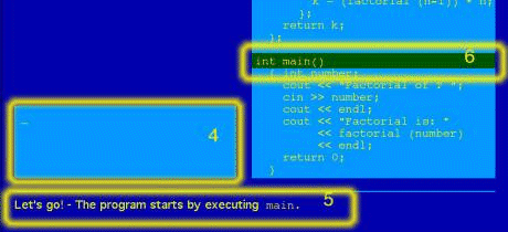
(In the above and the following figures the yellow frames and bold numbers are only for clarifying the references or for highlighting. They are not part of the animation.)

In the area 4, figure 2 shows (according to chapter 2(4)) the current status of the output of the program. Actually, you can only see the insertion point for output, represented by "-" . Area 5 shows a comment (cf. Chapter 2 (5)). In area 6 you can find the line, which is actually to execute, highlighted by a darkened background.

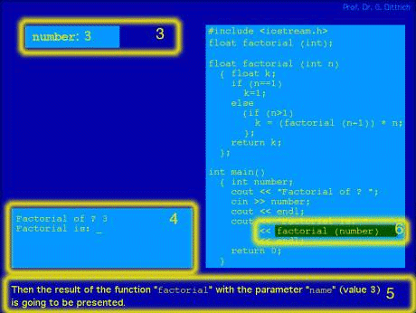
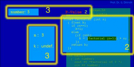
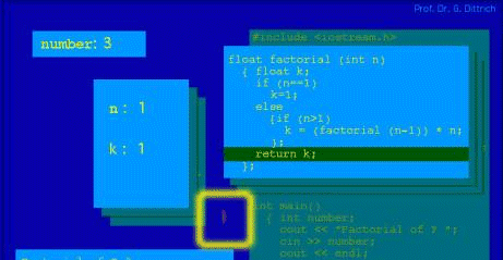
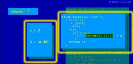
In Figure 3 we find the situation before execution of the function "factorial" with the current parameter 3. In addition to the explanations of 4, 5, and 6 (with the current information top left we find the current part of existing variables (according to chapter 2(3)). As can be seen, in order to gain insights in the global state of this situation, we have to look at 4 different distributed places.

Let us switch to the Figure 4. Figure 4 shows the situation, that the program is just before executing factorial for the second time, that is in this case with current parameter 2. Here the control is transferred to the first invocation of factorial. This is expressed by darkening the main program (cf. 2, as required in Chapter 2 (2)). The current state of the program is composed of the current value of the variable "number" of the main program, the current values of the local variables and the current parameter, here denoted as P-Value, for the next invocation of "factorial". You can find all this information explicitly.

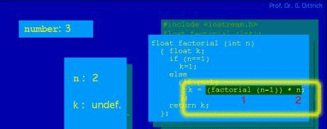
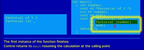
Figure 5 depicts the situation immediately after the second invocation. The shadowing of the code of the first invocation of the code is accompanied with a shadowing of the local variables. These two phenomena can be seen as represented in the parts 2 and 3, respectively.

As you know, in order to come to the terminating branch of "factorial" we need three invocations of the function in total. The main part of this situation after executing the third invocation can be found in Figure 6. Here we have stacked function invocations and local variables 3 times. The result of the last invocation is 1. Directly after this execution the instance of the third invocation will be removed uncovering the second invocation of "factorial" and leaving the result "1" for the call of factorial. This can be seen in figure 7. Now the calculation in the second instance of factorial can be executed. This situation can be found in Figure 8. In more steps similar to those represented in Figures 6 to 8 we can come back to the first call of factorial in the main program.

The situation there can be seen in Figure 9.

The very end is depicted in figure 10.

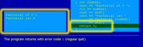
After looking at all these screenshots I hope the reader is convinced that all relevant aspects as mentioned in chapter 2 are really explicitly modeled thus leading to an easy understanding of the description of nontrivial issues.

With respect to this animation one may think to pursue the following alternative:

Run the program in a modern program developer tool in the debug mode (e.g. Project Builder under Mac OS X). This procedure has the big advantage that different programs can be explained in detail. Disadvantages are that on the one hand the stacking mechanism is a little bit difficult to understand and on the other hand that the presentation is not reproducible in a natural manner. The second drawback can be avoided by filming the display with a camcorder or by applying an appropriate program for catching the dynamic content of the display or parts of them (e.g. Snaps Pro under Mac OS X).

4 Conclusion

Using the example factorial(3) to introduce the mechanism of running programs with recursion we explained how to profit from representing dynamics by applying animations or similar time based media objects. The price we have to pay is the development of an appropriate mental model explicitly representing all relevant aspects of that what happens. The differences to other usually applied presentations are discussed a little bit.

Now we are only in a position to gather experience to present dynamics applying time based media objects by developing further different examples. We hope that in the near future this will lead to some sort of methodology in order to develop such documents.

References

[Dittrich 98] Dittrich, G.: "Rechnerunterstützte Informatiklehre: Ansätze zur Einbringung von Hypermedia-Elementen in den Hochschulunterricht" in Appelrath, H.-J. - Boles, D. - Meyer-Wegener (Edts.) Tagungsband WS Multimedia-Systeme, p. 19-30, 28. GI-Jahrestagung, Magdeburg, Sept. 1998 (in German)

[DittWest 00] Dittrich, G. - Westbomke, J.: "On Potential Areas of Multimedia-Application in Teaching and Learning at Universities", Article idpt99072 of IDPT2000 (International Conference on Integrated Design and Process Technology) Dallas, Texas, June 2000

[Dittrich 01] Dittrich, G.: "Einführung in die Informatik für Naturwissenschaftler und Ingenieure I, WS 2001/02, FB Informatik, Uni Dortmund, (in German) http://mediasrv.cs.uni-dortmund.de/Lehre/EINI-I_WS01_02/index.html (in German)

[DoberDiss 96] Doberkat, E.-E. - Dißmann, S.: Einführung in die objektorientierte Programmierung mit BETA, Addison-Wesley, 1996 (in German)