| Submission Procedure |
Fast Two-Stage Lempel-Ziv Lossless Numeric Telemetry Data Compression Using A Neural Network PredictorRajasvaran Logeswaran Abstract: Lempel-Ziv (LZ) is a popular lossless data compression algorithm that produces good compression performance, but suffers from relatively slow processing speed. This paper proposes an enhanced version of the Lempel-Ziv algorithm, through incorporation of a neural pre-processor in the popular predictor-encoder implementation. It is found that in addition to the known dramatic performance increase in compression ratio that multi-stage predictive techniques achieve, the results in this paper show that overall processing speed for the multi-stage scheme can increase by more than 15 times for lossless LZ compression of numeric telemetry data. The benefits of the proposed scheme may be expanded to other areas and applications. Keywords: Lempel-Ziv, neural networks, prediction, lossless compression, two-stage 1 IntroductionLossless data compression, emphasizing on the accuracy of compressed data, has many well known algorithms ranging from the primitive null suppression [Nelson 96], to well known statistical techniques such as Huffman [Huffman 52] and arithmetic coding [Langdon 84], and combination strategies, e.g. Sixpack, gzip, ARJ, LHA etc. [Nelson 96]. The popular Lempel-Ziv (LZ) [Ziv 77] dictionary algorithm scheme (and its many variants) traditionally produce good compression performance but at a relatively slow processing speed for use in many practical applications. This paper proposes using a neural network predictor in a two-stage scheme to speed-up the LZ implementation for lossless data compression. It is known that multi-stage predictive schemes [McCoy 94] improve compression performance dramatically, especially for data that contain repetative sequences or vary gradually. Using such an implementation, it is shown by the results in this paper that in addition to improved compression performance, the proposed scheme of incorporating a neural predictive pre-processor to the LZ is capable of increasing processing speeds significantly, even for numeric multi-distribution telemetric data. As LZ algorithms are widely used in many applications, a fast and improved implementation would have far-reaching benefits. In addition, its incorporation with yet another popular scheme of a predictive pre-processor (i.e. neural networks), and the significant merits gained through the combination, should prove beneficial for an even wider range of applications. Page 1199 2 Lempel-Ziv Algorithm BasicsA dictionary-type encoder builds a table of characters / words / phrases that have been encountered in the input stream, assigning a corresponding codeword to each entry in the table. When an instance in the input matches an entry in the table (dictionary), it is replaced with the corresponding codeword. Dictionaries may be static (pre-defined) or dynamic (built and updated at run-time, possibly initialised with pre-defined common matches at start-up). The LZ (also known as Ziv-Lempel and LZ77) [Ziv 77] has a text window divided into two parts : the body (containing recently encoded text), and a look-ahead buffer (that contains the new input to be compressed). The algorithm attempts to match the contents of the buffer to a string in the dictionary (body of text window), as shown in Fig. 1. Essentially, compression is achieved by replacing variable-length text with fixed sized tokens, each consisting of 3 parts : a pointer into the dictionary, the length of the phrase and the first symbol in the buffer that follows the phrase (example, Fig. 1(b)). The token is read, the indicated phrase is output and the remaining character is appended. The process is repeated until the end of the input. BODY OF TEXT
WINDOW
LOOK AHEAD BUFFER
(a) LY77 Text window at a particular instance (above).
(b) Match Found: Text window and look-ahead buffer shifted left by 3
places after LZ77 encoding
(c) No Match: Text window and look-ahead buffer shifted left by 1
place
after LY77 encoding of '+'. Note: Token format =
[position of match, length, next charakter] Figure 1: Example of Lempel-Ziv Coding (LZ77) The implementation of LZ77 can cause a bottleneck due to relatively
slow string comparison that has to be done at every position in the
text
window. When matching strings are not found, the compression cost of
using
this algorithm is high as the 24-bit token (three 8-bit characters) is
used to encode each unmatched 8-bit character (see
Fig. 1(c)). Many
improved
variants of the LZ class of algorithms have been created, including
LZSS,
LZ78, LZW, LZJ, LZT, LZC, LZH and LZARI [Nelson 96],
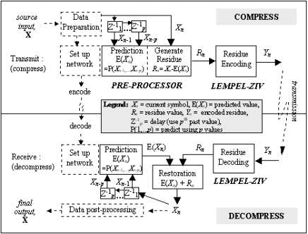
[Storer 82], [Ziv 78]. Two LZ variations are implemented in this paper. LZSS [Storer 82] updates a binary search tree with the phrases moved out of the buffer into the dictionary, allowing quick string comparison, thus reducing the performance bottleneck. Page 1200 Wastage is reduced by modifying the token to use a 1-bit prefix to indicate whether an offset (length pair, e.g. 17-bit token [0, (11,3)]) or a single symbol (e.g. 9-bit token [1, '+']) is sent as output. When unmatched, the dummy position 0 and length 0 will not be sent, thus saving 15 bits as compared to the implementation in Fig. 1(c). LZARI [Nelson 96] is a multilevel coding technique that uses a two-pass operation - the first uses one of the better LZ algorithms, followed by arithmetic coding [Langdon 84] of the tokens (code pointers). 3 Enhanced Two-Stage Lempel-ZivThe proposed two-stage LZ scheme integrates a predictor (coupled with a residue generator) as a pre-processor to the LZ encoder, as shown in Fig. 2. The 1st stage is a pth order predictor which reduces the dynamic range of the input by predicting the current input value (Xn) at each iteration, and outputs the corresponding residue, Rn = Xn - E(Xn), which is then LZ encoded in the 2nd stage to produce the transmitted compressed residue (Yn). Figure 2: Two-stage Scheme 4 Performance ResultsThe simulation model in Fig. 3 is set up for performance evaluation, catering for the training requirements of the pre-processor to allow for adaptive prediction of the varying input patterns. A variety of predictors are evaluated, as described in Section 4.2. As the LZ algorithm has undergone many improvements over the years since its conception, the popular LZSS and LZARI are used instead of the original LZ77, for a more realistic implementation. As LZARI is already a multi-stage encoder, its use is suitable for also studying the performance effects of further incrementing the number of stages in an algorithm. Page 1201 Figure 3: Implementation schematic of the two-stage scheme 4.1 Test DataEvaluation of the scheme is carried out with a data set of typical
1-D
numeric telemetry data files acquired from the various sensors aboard
satellite
launch vehicles, which contain data of varying magnitude and mixed
distribution
patterns. General characteristics of the test files are provided in
Tab. 1 [Rahaman 97].
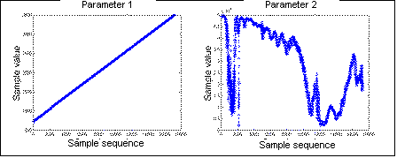
Table 1: Characteristics of the test data files Page 1202 Each test file consists of pairs of values - the first parameter
being
a reference value (e.g. coordinates, time etc.) with semi-linear
distribution,
and the latter the actual measurement of varying distributions, as
signified
by the frequency and entropy (H = - Figure 4: Distribution of the separate parameters of test file tdata5 4.2 Pre-processor Predictor SelectionA variety of predictors may be used in the 1st stage. The results for some classical and artificial neural network (ANN) predictors evaluated are given in this paper, namely: ANN - 4th-order single layer perceptron (SLP) and 3rd-order multi-layer perceptron (MLP) with 2 hidden nodes [Logeswaran 01]; Classical - 5th-order fixed FIR filter, adaptive FIR with normalized least mean squared (NLMS) algorithm and 2-layer recursive least squares lattice filter with a-priori estimation errors and error feedback (RLSL) [Haykin 91], [McCoy 94]. Tests with other predictors were found to produce similar conclusions [Logeswaran 02]. The ANN were trained using the common Backpropagation with a learning rate of 0.1. The topology of the pre-processors setup were intentionally unoptimized to test the scheme for simple implementation on small encoders with minimal overheads. To handle the dual distribution of the test data, two predictors are used in the 1st-stage - one per parameter, to produce the best match of the input pattern. The output of the 1st stage is interleaved such that the output (i.e. input to the LZ encoder in the 2nd stage) is again pairs of numbers of residues of the parameters, in the sequence of the original input files. NLMS and RLSL are fully adaptive algorithms, retrained (adaptive coefficients) as each new value is presented. For the ANN, training is conducted via a block-adaptive technique [Logeswaran 02], where the incoming input is split into blocks and the networks are retrained on-the-fly for each block using the first 20% of samples in the block. This technique prevents the over-fitting of the ANN (thus preventing rigid predictors), yet allows some adaptability to the input patterns. The static FIR filter is non-adaptive and requires no training - its coefficients are determined experimentally [McCoy 94]. Page 1203 4.3 Processing Time ResultsThe processing time of the encoders in the single-stage (LZ only)
and
two-stage (predictor-LZ combination) schemes is summarized in Tab. 2.
It
is shown that the processing time of the LZSS and LZARI by themselves
is
large (more than 8 seconds), but is significantly reduced (down to 5.41
% of the original time) when the pre-processing stage is introduced,
making
the proposed multi-stage implementation faster by up to 17.5 times. The
training times are not included in the table as in conventional
implementations,
the predictors would be intitialized to optimum settings, and adaptive
training is handled concurrently during the prediction process.
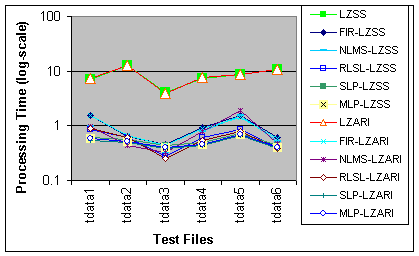
From Fig. 5, it is observed that the
processing time for the LZSS
and
LZARI (and their two-stage schemes) are similar, but processing time
achieved
vary between the type of predictors used, where the ANN schemes are
seen
to perform better than the classical predictors. It is also important
to
note that through the use of the pre-processor, the total processing
time
for the different files are relatively consistent and low, as opposed
to
the large differences observed for the LZ-only implementations across
the
different distribution patterns in the test files. These patterns do
also
affect predictors in the two-stage scheme, but as the chosen predictors
are fast and take up only approximately 0.2-0.3 seconds in processing
time,
the influence on overall performance of the two-stage scheme is
minimal. Page 1204 Figure 5: Processing time achieved by the encoder-only and two-stage schemes for the different test files
Table 3: Processing time (seconds) for each parameter compressed
separately using only the LZ algorithm Page 1205
Incidently, results of processing the individual parameters separately are given in Tab. 3 to compare the LZ performance for the different types of distribution of the input parameters. Whilst the results in Tab. 2 show similar total processing times by both the LZSS and LZARI schemes, Tab. 3 shows that there is significant difference in speed when the parameters are treated separately. The split allows much faster encoding of the each parameter and in the total processing time as a whole, more so in LZSS than in LZARI. The separate parameter implementation works faster since the matches in the dictionary are located faster as the dictionary for each parameter is smaller than the whole put together. The results also suggest that there are more unique values in the 1st parameter (based on higher processing time) than in the 2nd parameter, in accordance with Tab. 1. In the case of LZARI, being multi-stage (LZ with arithmetic coding), it has larger intrinsic overheads, thus its gain in processing speed is comparably less than that of the LZSS.
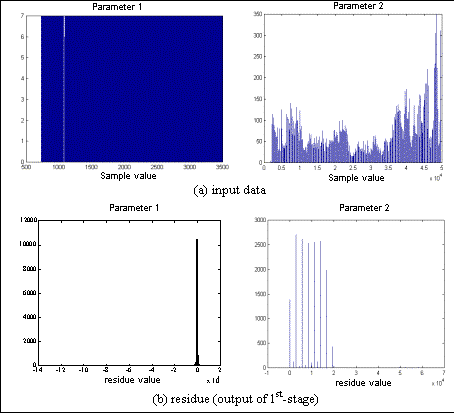
Table 4 : Compression ratio performance achieved by LZ and LZ two-stage schemes 4.4 Compression Performance ResultsWhen dealing with compression, it is important to ensure high compression ratios (CR) are obtained. The results in Tab. 4, in terms of CR achieved for each test file, show that the two-stage scheme produces significant improvement in compression, as expected from a multi-stage implementation. In the case of the fixed FIR, compression performance deteriorates because the fixed predictor is not able to cope with the input pattern well and produced large residues with low frequency distribution, thus requiring larger codewords and causing data expansion (where the resulting CR are less than those achieved by the single stage LZSS and LZARI implementations). The other two-stage schemes performed well, with the classical RLSL producing the best results for LZSS and the ANN MLP the best for LZARI, obtaining CR of above 40. In addition, as with the experiment for processing time, each parameter was coded separately using the LZ algorithms, but no performance gains in terms of CR was achieved due to the very little overlap between the values of the 1st and 2nd parameters. The number of entries in the dictionary were not observably affected, and neither were the codewords nor the total compression performance. Page 1206 5 DiscussionThe compression performance results achieved for the multi-stage scheme was higher, as expected. However, the performance of the proposed schemes in terms of processing time is rather surprising, especially as it was significantly faster despite the addition of an additional stage to the LZ algorithm. This was possible as the output of the 1st stage is a binary stream in which each input value (Xn) is represented by a residue (Rn) that is generally significantly smaller in magnitude than Xn. The LZ algorithms used assume input of 16-bit integers, whilst each symbol in the residue stream is r. bits (residue word size, can be as low as 2 bits long, the 1st being a sign bit). In effect, in the two-stage scheme, the LZ algorithms process a number of residue symbols at a time to make up the 16 bits, so the total number of iterations of the LZ algorithm is reduced, thus speeding up processing. A good predictor removes redundancy in the input such that the probability density function of the residues has a mean of 0 and a small standard deviation. As the range of values of Rn is small, the number of unique patterns passed on to the encoder is minimal. The LZ benefits from the reduced size dictionary / lookup table it needs to build and use to store these patterns. The processing time for building, lookup and and associated I/O processes involved with the dictionary, and in producing output, is thus dramatically reduced, especially for long streams of similar residues values. As such, the total processing time is significantly reduced through the introduction of a good predictive pre-processor. A frequency histogram may be plotted to illustrate the performance of the predictor, and the proposed implementation. Fig. 6 shows that the number of unique values of data is dramatically reduced, supported by the significant increase in frequency of a few values (e.g. from a maximum frequency of 7 per symbol to a frequency above 10000 for residue value 0 in the first parameter, and from an average frequency of about 100 to above 2500 for certain residue values in the second parameter). Improving the predictor implementation would enable the pre-processor to achieve an even smaller range of Rn, and improve the compression performance further. The above observations also explain the increases in the compression ratio gained by the proposed scheme as a smaller number of symbols are encoded, and a smaller number of tokens are output. Since the LZ algorithms do not utilize the distribution pattern of the input directly, but rather the actual Xn values, the predictor pre-processor complements it well and produces the marked performance increase in terms of processing time and compression ability achieved. Page 1207 Figure 6: Frequency histogram of input and the generated residue values of the separate parameters of file tdata5 The performance of the two-stage scheme is subject to certain overheads. Additional processing power and machine cycles are needed in the 1st stage, along with buffer space for storing the p past values. Adaptive predictors require resources for training, thus causing a slight increase in processing time. Identical predictors must be set up at both the transmitter and receiver ends in order to produce the identical predicted values that will be added to the residue to restore the original input values. Certain set up information, such as the number of parameters, pseudo-random generator key, chosen training algorithm, initial p value to initiate prediction etc. may need to be transmitted as preamble for implementation of flexible predictors. Such implementation may reduce the compression performance slightly, depending on the available resources and amount of hardware and software customisation and flexibility required. In most cases, a system for data compression tends to have a specific application (e.g. in transmitting telemetry data for a certain application frome a remote sensor) and such dedicated systems would be customised, incurring minimum processing and setup overheads. Page 1208 Implementing a dynamic residue size for each residue value is costly as there has to be an indicator of the number of bits to be read at the receiver end to restore the value. To minimize this overhead, past experience with similar types of data is used to select an "optimum" word-size (r bits) for the residues (e.g. 3 bits), as undertaken in this simulation. If a residue requires a larger word-size (e.g. in the event of signal impulse or very irregular input values), the residue is discarded. Instead, the actual input value (v bits) is transmitted preceded by an r bit flag (e.g. -0, zero with the sign bit set to negative). Each value transmitted is either v or r bits, thus minimizing the chances of data expansion (although expansion occurs if r is chosen poorly as many flags would be transmitted). It must also be noted that the test data sets used were numeric telemetry data, which is not best suited for LZ compression. The intentional use of such data was to portray a non-optimum scenario for displaying the capabilities of the LZ algorithms in compressing such numeric data, and for ease of implementation of the predictors. The data chosen was also dual parameter and of varying distribution to better test the proposed scheme, as the input values would not follow a predictable sequence due to the interleaving of the dramatically different parameter values. For general-purpose testing, standard test sets such as those in the cantebury corpus may be used. In addition, the predictors used were of low complexity (only containing less than 5 nodes) for practical implementation of small systems (which would be expected for remote sensors acquiring the telemetry data). The adhoc training mechanism used was to present the predictors with incoming data on-the-fly, training with just the first 20% of a block of data. Such testing of the system with no prior knowledge of the data (through random initialization) was undertaken to simulate a robust implementation that learns and adapts to non-standardized input. In conventional systems, there is usually an abundance of past data and systems usually need to only cope with a limited set of input patterns. As such, initializing the predictor through preparation of a proper training dataset containing a good sample of various expected input (and target, for supervised training) patterns, extracted through feature analysis, would certainly enable the predictor, and thus, the two-stage scheme to preform better. 6 ConclusionIn this paper, a two-stage scheme is successfully implemented to improve the performance of the Lempel-Ziv (LZ) dictionary-type lossless compression algorithm. The method employed is via integration of a predictive pre-processor stage with the LZ algorithm. Tests conducted with a number of classical and neural predictors, with two LZ algorithms, shows that the multi-stage predictive LZ scheme can significantly speed up processing in addition to improving compression performance. The simulation results for some small known predictors show that processing speeds of up to almost 18 times faster, with compression ratio of more than 45 can be achieved by the proposed two-stage scheme as compared to single-stage LZ-only implementations. Performance (compression as well as speed) relies on the combination of both stages, so the suitability of the predictor in generating an appropriate residue stream for the particular LZ encoder must be mentioned [Logeswaran 01], [Logeswaran 02]. Page 1209 Through empirical or analytical means, the number and type of pre- (and possibly post-) processing stages used could be determined by the overall performance gains versus the resources requirements for the additional integration. The generalized scheme presented here may be expanded to larger systems and is expected to produce better results with the use of customised predictors. The results recommend that with a suitable pre-processor stage, performance of the encoder can be improved significantly, when dealing with different data. This is true not just for the test set of telemetry data used in this paper, selected for their varying paterns in data distribution, but for any data that has patterns in the input that may be predicted. Based on the popularity of the LZ algorithms and the predictor-encoder schemes, the proposed scheme may prove beneficial for a large domain of applications. It is also noteworthy that ANNs tend be faster and more error tolerant than their classical counterparts [Logeswaran 00], making then also the more suitable predictors for critical systems. Acknowledgements The author acknowledges the contributions and guidance of Prof. C. Eswaran and M.U. Siddiqi of Multimedia University, Malaysia in conducting this work. References[Haykin 91] Haykin, S.: "Adaptive filter theory"; Prentice Hall International, New Jersey (1991) [Huffman 52] Huffman, D.A.: "A method for the construction of minimum redundancy codes"; Proc. of the IRE, 40 (1952), 1098-1101. [Langdon 84] Langdon, G.G.: "An introduction to arithmetic coding"; J. IBM R&D (1984) [Logeswaran 00] Logeswaran, R. and Siddiqi, M.U.: "Error Tolerance in Classical and Neural Network Predictors"; IEEE TenCon, 1 (2000), 7-12 [Logeswaran 01] Logeswaran, R. : "Transmission Issues of Artificial Neural Networks in a Prediction-based Lossless Data Compression Scheme"; IEEE Int. Conf. on Telecommunications, 1 (2001), 578-583 [Logeswaran 02] Logeswaran, R.: "A Prediction-Based Neural Network Scheme for Lossless Data Compression"; IEEE Trans. on Systems, Man, and Cybernetics - Part C: Applications and Reviews, 32, 4 (2002), 358-365 [McCoy 94] McCoy, J.W., Magotra, N. and Stearns, S.: "Lossless predictive coding"; IEEE Midwest Symp. on Circuits and Systems (1994), 927-930 [Nelson 96] Nelson, M. and Gailly, J.L.: "The data compression book"; M&T Books, New York (1996) [Rahaman 97] Rahaman, F.: "Adaptive entropy coding schemes for telemetry data compression"; Project Report No. EE95735, Indian Institute of Technology, Madras, India (1997) Page 1210 [Storer 82] Storer, J.A. and Szymanski, T.G.: "Data compression via textual substitution"; J. ACM, 29, 4 (1982), 928-951 [Ziv 77] Ziv, J. and Lempel, A.: "A universal algorithm for sequential data compression"; IEEE Trans. on Information Technology, 23, 3 (1977), 337-343 [Ziv 78] Ziv, J. and Lempel, A.: "Compression of individual sequences via variable-rate coding"; IEEE Trans. for Information Technology, 24, 5 (1978), 530-536 Page Page 1211 |
|||||||||||||||||||||||||||||||||||||||||||||||||||||||||||||||||||||||||||||||||||||||||||||||||||||||||||||||||||||||||||||||||||||||||||||||||||||||||||||||||||||||||||||||||||||||||||||||||||||||||||||||||||||||||||||||||||||||||||||||||||||||||||||||||||||||||||||||||||||||||||||||||||||||||||||||||||||||||||||||||||||||||||||||||||||||||||||||||||||||||||||||||||||||||||||||||||||||||||||||||||||||||||||||||||||||||||||||||||||||||||||||||||||||||||||||


 Pi log2 (Pi
) information in

