Computational Geometry - Some Easy
Questions and their Recent Solutions
Franz Aurenhammer
(Graz University of Technology, Graz, Austria
auren@igi.tu-graz.ac.at)
Abstract: We address three basic questions in computational geometry
which can be phrased in simple terms but have only recently received (more
or less) satisfactory answers: point set enumeration, optimum triangulation,
and polygon decomposition.
Key Words: Computational geometry, combinatorial geometry, point
set data base, minimum-weight triangulation, polygonal skeleton
Categories: F.2.2
1 Introduction
Computational geometry is concerned with the algorithmic study of elementary
geometric problems. Ever since its emergence as a new branch of computer
science in the early 1970's, a fruitful interplay has been taking place
between combinatorial geometry, algorithms theory, and more practically
oriented areas of computer science. Computational geometry has been among
the driving forces for developing advanced algorithmic techniques, data
structures, and settheoretic concepts. Parametric search, randomization,
planesweep technique, fractional cascading, and  nets are a some examples.
On the other hand, interest has been renewed in elementary geometric and
graphtheoretic concepts, like convex hulls, arrangements, Voronoi diagrams,
triangular networks, and hypercubes. A fact which maybe fascinates many
computational geometry researchers (including the author) most is that
many questions in this area, which may have deep and complex answers, can
be stated in an extremely simple and elegant way. The present paper is
devoted to some questions of this kind. Choice is rather subjective than
representative, and is mainly guided by the author's topics of interest
within the past few years. nets are a some examples.
On the other hand, interest has been renewed in elementary geometric and
graphtheoretic concepts, like convex hulls, arrangements, Voronoi diagrams,
triangular networks, and hypercubes. A fact which maybe fascinates many
computational geometry researchers (including the author) most is that
many questions in this area, which may have deep and complex answers, can
be stated in an extremely simple and elegant way. The present paper is
devoted to some questions of this kind. Choice is rather subjective than
representative, and is mainly guided by the author's topics of interest
within the past few years.
2 Which Sets of 10 Points Do Exist
A set of n points in the plane is the underlying structure for various
problems in computational geometry. In fact, a finite set of points seems
to be among the simplest geometric objects that lead to nontrivial
geometric and algorithmic
questions. Not surprisingly, most of the basic concepts and data structures
in computational geometry have first been developed for point sets and
later been generalized to more general objects like line segments, circles,
polygons etc. Examples include the convex hull, the Voronoi diagram, and
geometric search trees, just to name a few.
Quite a large subclass of problems is determined already by the 'combinatorial'
properties of an npoint set S rather than by its metric
properties. More precisely, look at all the  straightline segments
spanned by the points in S. The way these segments cross each other
turns out to be of importance, in the sense that point sets with identical
crossing properties give rise to equivalent geometric structures. This
is true for many popular structures like spanning trees, triangulations,
polygonalizations, socalled ksets, and many others. straightline segments
spanned by the points in S. The way these segments cross each other
turns out to be of importance, in the sense that point sets with identical
crossing properties give rise to equivalent geometric structures. This
is true for many popular structures like spanning trees, triangulations,
polygonalizations, socalled ksets, and many others.
Several of these structures lead to hard problems. For some of them,
like counting the number of triangulations of a given point set, no subexponential
algorithms are known [1]. For others, like for ksets,
the combinatorial complexity is still unsettled [21].
Sometimes even the existence of a solution has not yet been established,
such as the question of whether any two given npoint sets (with
the same number of extreme points) can be triangulated in an isomorphic
manner [5]. To gain insight into the structure of hard
problems, examples that are typical and/or extreme are often very helpful.
To obtain such examples usually complete enumerations on all possible
problem instances of small size are performed. In our case this means to
investigate all 'different' sets of points, where diffence is with respect
to the crossing properties of the sets. This leads us to questions like,
'Which sets of, say 10, points do exist?'. The answer is surprisingly difficult,
due to two reasons. First, the number of inequivalent point sets of size
10 is already in the millions (14 309 547, to be precise). Second, there
seems to be no simple way to enumerate all these sets, because each increase
in size gives rise to types which cannot be obtained directly from sets
of smaller size. This may explain why it took until recently that the first
complete data base on 10point sets has been established; see Aichholzer
et al. [7]. Below we describe, in a more formal style,
the inherent difficulties of such a project, along with first applications
and results obtained from the 'point set data base'.
2.1 The approach
An appropriate tool to reflect the crossing properties of a given
point set has been developed quite a while ago. Goodman and Pollack
[27] introduced the order type of a set
{p1 , ... pn } of points as a
mapping that assigns to each ordered triple i, j,
k in {1, ... , n} the orientation (either clockwise or
counterclockwise) of the point triple pi,
pj, pk. Two point sets
S1 and S2 are said to be
equivalent if they exhibit the same order types. That is,
there is a bijection between S1 and
S2
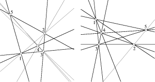
Figure 1: Two equivalent sets of 5 points
such that any triple in S1 agrees in orientation with
the corresponding triple in S2; see Figure 1 for an example.
It is not hard to see that two line segments spanned by S1
cross if and only if the corresponding segments for S2
do. The goal is to enumerate all order types of size 10 (and less).
To this end, use can be made of the duality1
between point sets and line arrangements in the Euclidean plane. A line
arrangement is the dissection of the plane induced by a set of n straight
lines. As no direct way to enumerate these structures is known, we first
produce all nonisomorphic arrangements of socalled pseudolines.
A set of pseudolines is a set of simple curves which pairwise cross
at exactly one point. Handling pseudolines is relatively easy in view of
their equivalent description by wiring diagrams; see, e.g., Goodman [26].
Consult also Figure 2. We can read o a corresponding
pseudo order type from each pseudoline arrangement, because the
intersection orders on all the pseudolines uniquely determine the orientations
of all element triples. Back in the primal setting, where each line potentially
corresponds to a point, this leads to a list of candidates guaranteed to
contain all different order types.
This leaves us with the problem of identifying all the realizable
order types in this list, that is, those which can actually be realized
by a set of points. Here we enter the realm of oriented matroids
, an axiomatic combinatorial abstraction of geometric structures introduced
in the late 1970s. As a known phenomenon, a pseudoline arrangement need
not be stretchable, i.e., isomorphic to some straight line arrangement.
There exist nonstretchable arrangements already for 8 pseudolines;
see, e.g., Björner et al. [15]. As a consequence,
our candidate list will contain nonrealizable pseudo order types. Moreover,
even if realizability has been decided for a particular candidate, how
can we find a corresponding point set?
1Any of the wellknown
duality transforms used in computational geometry may serve this purpose,
although none of them leads to a bijection in order type.
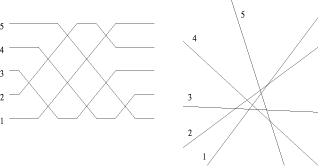
Figure 2: A wiring diagram that can be stretched
As a matter of fact, the situation gets conceptually and computationally
easier in the projective plane where unlike in the Euclidean plane
inequivalent order types directly correspond to nonisomorphic line arrangements,
and isomorphism classes of pseudoline arrangements coincide with (reorientation
classes of) rank 3 oriented matroids. For size 10, there exist exactly
312 356 classes of these matroids, 242 of which are nonrealizable; see
[15, 26]. This knowledge can
be put to use for our purposes in the following way.
Let  be the candidate list of order types obtained from wiring diagrams
(as sketched above). We group the members of into equivalence classes
by correspondence to the same projective order type. In every class, either
each or no order type is realizable. We know from matroid theory that P10
= 312 114 projective classes have to be realizable. Now, for each member
of , we try to recover a realizing point set. A counter is kept for the
number of realizable projective classes all of whose members have been
realized already. The process is terminated when this number reaches P10. be the candidate list of order types obtained from wiring diagrams
(as sketched above). We group the members of into equivalence classes
by correspondence to the same projective order type. In every class, either
each or no order type is realizable. We know from matroid theory that P10
= 312 114 projective classes have to be realizable. Now, for each member
of , we try to recover a realizing point set. A counter is kept for the
number of realizable projective classes all of whose members have been
realized already. The process is terminated when this number reaches P10.
Recovering realizing point sets is done by a combination of
heuristics, in cluding insertion stategies and simulated
annealing. To our fortune, one or the other heuristic eventually
succeeded in realizing all candidates which are indeed realizable. To
enhance the userfriendliness of the obtained data base, each
point set was postprocessed to fit into a small and nice grid
representation. Even this issue is by no means trivial, as a
doublyexponential lower bound on the required grid size is known;
see [28].
Table 1 lists the numbers of Euclidean order types according to the
size h of the convex hull of the realizing npoint sets.
It took 36 hours on a 500 MHz Pentium III to generate all Euclidean
pseudo order types of size n = 10, and to find realizing point sets
for all but some 200 000 of them, by using the insertion strategy.
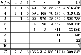
Table 1: Number of Euclidean order types classified by
extreme points
However, most of the projective classes corresponding to the
pseudo order types left unrealized got at least one member realized, and
could be completed quickly by a rotation technique. In particular, only
251 projective classes remained without any realized member. For these
classes, we had to invoke a simulated annealing routine, as we had no information
on which are the 242 classes known to be nonrealizable from literature.
We were successful for 9 classes within 60 hours whichfinally completed
this task.
Much additional effort has been required to obtain compact grid representations
for the realizing point sets, as well as for checking reliability of the
data base. In summary, a complete, userfriendly, and reliable data base
for all order types of sizes n  10 has been obtained. The data
base is made public on the web2. Due to
space limitations, the grid point sets of size 10 are not accessible online
but rather have been stored on a CD which is available upon request. 10 has been obtained. The data
base is made public on the web2. Due to
space limitations, the grid point sets of size 10 are not accessible online
but rather have been stored on a CD which is available upon request.
2.2 Some applications
Let us now briefly point out some situations were the complete enumeration
of all order types for n 10 leads to results for general problem
size n.
The obvious case is when a counterexample can be provided that generalizes
to larger n. There might exist counterexamples too large to be found by
hand though small enough to be detected by checking all order types. On
the other hand, the nonexistence of small counterexamples gives some evidence
for the truth of a conjecture.
As another example, case analyses for problem instances of constant
size are often encountered when proving some combinatorial property. This
is particularly true for induction proofs if a sufficiently large induction
base is sought. The point is that the quality of the initial values affects
the asymptotic behavior of the result.
2at http://www.igi.TUGraz.at/oaich/triangulations/ordertypes.html
It would lead to far to give concise definitions of all the problems
having been examined by means of the data base so far; we refer to [9]
instead. Complete enumerations have been done for frequently arising concepts
like triangulations, crossingfree Hamiltonian cycles, crossingfree spanning
trees, crossingfree matchings, ksets, and others. Extremal values
have been calculated for the crossing number (of the complete geometric
graph), the cover number and the partition number (by convex polygons),
the size of crossing families (in the complete geometric graph), the reflexivity
number (for Hamiltonian cycles), and more. In various cases, new results
and answers to open problems and conjectures have been obtained.
In conclusion, we believe that knowing 'which sets of 10 points do exist'
will be of use to many researchers in computational and combinatorial geometry
who wish to examine their conjectures on small point configurations.
3 Finding the Best Triangular Network
Generating quality triangular meshes is one of the fundamental problems
in computational geometry and has been studied extensively, from both the
theoretical and practical point of view; see e.g. the survey paper by Bern
and Eppstein [14]. Main fields of application include
finite element methods and computer aided design. In formulating a triangulation
problem, a choice arises between two types of triangulations: ones that
have exactly the input points as their vertices, and others where additional
points may be placed to increase quality. While the latter type probably
has received more attention in practice, the former type { triangulating
a fixed set of points 'optimally' { has attracted the interest of many
theoreticians. In fact, finding optimal triangulations is a hard problem,
apart from a few exceptions.
3.1 Optimal triangulations
Let us put the triangulation problem more formally. Let S be
a set of n points in the plane, and let E(S) be the
set of all (straightline) edges spanned by the points in S. A triangulation
of S is a maximal set of noncrossing edges from E(S).
Such a set of edges partitions the convex hull of S into triangles.
The number of different triangulations of S is an exponential function
of n; see [8]. This fact already indicates that
constructing optimal triangulations in polynomial time might be a challenging
task. This becomes more apparent as common greedy methods, like deleting
candidate edges or triangles from worst to best, are doomed to fail by
the NPcompleteness of the following problem; see Lloyd [32]:
given some subset of E(S), decide whether this set contains
a triangulation of S.
Results on optimizing combinatorial properties of triangulations,
such as maximum vertex degree or connectivity are rare. Most optimization
criteria where efficient algorithms are known concern the geometric
properties of the edges and triangles. The interested reader may consult
the recent survey article by Aurenhammer and Xu [12]
on optimal triangulations.
The most commonly constructed, and maybe the most famous triangulation
for a point set S is the Delaunay triangulation, DT(S).
See e.g. [24, 11] for extensive
treatments. DT(S) contains for each triple of points in S
the corresponding triangle, provided its circumcircle is empty of points
in S. Various global optimality properties of DT (S)
can be proved by observing that certain edge flips (exchanges of
diagonals) yield a local improvement of the respective optimality measure.
For example, equiangularity of a triangulation, which is the sorted
list of its angles, increases lexicographically in this way. DT(S)
thus maximizes the minimum angle. This is one of the main reasons why the
Delaunay triangulation is the structure of choice in various practical
applications: small angles are a potential source of numerical errors in
many computations. Another reason for the popularity of DT (S) is its low
computational complexity; several simple O(n log n)
construction algorithms exist. DT(S) also minimizes, among
other quality criteria, the largest circumcircle that arises for the triangles,
and it maximizes the sum of triangle inradii. On the negative side, DT(S)
fails to fulfill optimization criteria similar to those mentioned above,
such as minimizing the maximum angle, or minimizing the longest edge.
3.2 Minimumweight triangulation
Most longstanding open is another optimal triangulation problem: what
is the 'shortest possible' triangulation of a point set S ? More formally,
for the minimum weight triangulation the optimization criterion is weight,
which is defined as the sum of all edge lengths. The complexity of computing
a minimum weight triangulation, MWT (S), for arbitrary planar point sets
S is still open since 1975 when it was mentioned in Shamos and Hoey [34].
Minimum weight triangulation is included in Garey and Johnson's [25]
list of problems neither known to be NPcomplete, nor known to be solvable
in polynomial time. Attempts to prove the problem NPhard have resulted
in some related NPcompleteness results. Several heuristic algorithms have
been proposed to solve this problem. However, only recently progress has
been made to produce a constant approximation in weight. (For more details
on these and the following properties of minimum weight triangulations
see, e.g., [12].)
Among others, dynamic programming approaches and linear programming
techniques have been tried. The former works in O(n3)
time if the underlying point set S is the set of vertices of a simple
polygon. This fact gave motivation
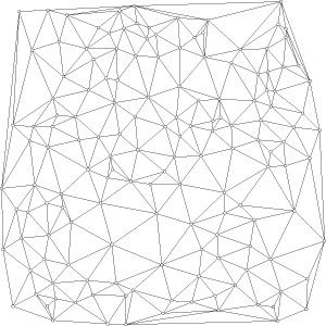
Figure 3: Minimumweight (light) triangulation for 150
points
for the following subgraph approach to compute MWT(S).
First, find a (suitable) subgraph G of MWT(S). If
G contains k connected components, try all possibilities
to add k 1 edges to make it a connected graph C. Complete
each of these graphs C to a triangulation by optimally triangulating
its faces, and select a triangulation with minimum weight, which gives
MWT(S). This approach, which basicly is exhaustive search,
can be implemented to run in O(n k+2) time. The
problem, of course, is to find candidate subgraphs G with k
small, preferably constant.
Many efforts have been put into the investigation of subgraphs of MWT
(S). Still, only in recent years have several nontrivial subgraphs
of MWT(S) been identified. One of them arises from a class
of empty neighborhood graphs called  skeletons. An edge between points
p, q skeletons. An edge between points
p, q  S belongs to the skeleton of S if the
two circles of diameter S belongs to the skeleton of S if the
two circles of diameter  |pq| and passing through both p
and q are empty of points in S. This skeleton happens to
be subgraph of MWT(S) for large enough, as has been observed
first in Keil [29]. Unfortunately though, the resulting
graph may be highly disconnected. |pq| and passing through both p
and q are empty of points in S. This skeleton happens to
be subgraph of MWT(S) for large enough, as has been observed
first in Keil [29]. Unfortunately though, the resulting
graph may be highly disconnected.
A distinct attempt to find a sufficient local condition defines an edge
e E(S) as a light edge if there is no edge
in E(S) which crosses e and is shorter than e. Let
L(S) denote the graph formed by all the light edges for S.
The interesting property is the following: if L(S) happens
to be a full triangulation of S, then L(S) = MWT(S).
This allowed, for the first time, for a fast computation of
MWT(S) for a nontrivial class of point sets of moderate
size; see Figure 3.
This result is a consequence of the following matching theorem
for planar triangulations, proved independently in Aichholzer et al. [6]
and in Cheng and Xu [18]: for any two triangulations
T1 and T2 of a fixed point set S,
there is a perfect matching between the edge set of T1
and the edge set of T2 such that matched edges either
cross or are identical.
3.3 The LMT-skeleton
So far, we have seen that several subgraphs of MWT(S)
can be found from some local conditions. Still, we are far away from an
algorithm for computing MWT (S) that works efficiently for
general point sets S. The breakthrough (at least from the practical
point of view) came from considering subgraphs which are defined in a global
way, in the following surprisingly simple manner.
Call a triangulation T of S locally minimal if
every pointempty and convex quadrilateral drawn by T is optimally
triangulated (that is, contains the shorter of its two diagonals). Let
LMT(S) denote the intersection of all locally minimal triangulations
for S. Then LMT(S) is a subgraph of MWT(S),
as this triangulation of course is locally minimal, too.
Whereas it is not known how to compute LMT(S) in polynomial
time, a surprisingly large subgraph of LMT(S), the socalled
LMTskeleton, can be identified by the simple method below, recently
proposed in Belleville et al. [13] and in Dickerson
and Montague [22]. Consider some edge set E  E(S). An edge e E is called redundant
in E if there is no convex quadrilateral formed by E that
has e as its shorter diagonal. Edge e is called unavoidable
in E if no other edge in E crosses e. The LMTskeleton
algorithm puts E = E(S) and proceeds in several rounds.
Each round first identifies all edges redundant in E and eliminates
them from the set, and then includes into the LMTskeleton all edges that
are unavoidable in the reduced set E. The algorithm stops when no
more edges in E can be classified as either redundant or unavoidable.
The number of rounds (but not the produced LMTskeleton) depends on the
ordering in which the edges are examined. E(S). An edge e E is called redundant
in E if there is no convex quadrilateral formed by E that
has e as its shorter diagonal. Edge e is called unavoidable
in E if no other edge in E crosses e. The LMTskeleton
algorithm puts E = E(S) and proceeds in several rounds.
Each round first identifies all edges redundant in E and eliminates
them from the set, and then includes into the LMTskeleton all edges that
are unavoidable in the reduced set E. The algorithm stops when no
more edges in E can be classified as either redundant or unavoidable.
The number of rounds (but not the produced LMTskeleton) depends on the
ordering in which the edges are examined.
The fact that the LMTskeleton for a point set S, and thus LMT(S),
tend to be connected even for large point sets comes as a surprise. From
the practical point of view, the LMTskeleton almost always nearly triangulates
S; cf. Figure 4. On the other hand, a 19point counterexample to
connectedness exists [13]. Moreover, even for uniformly
distributed points, the expected number of components is  (n); see
[16]. (The constant of proportionality is extremely
small, though.) It is interesting to note that the LMTskeleton, and the
graph of light edges L(S), exhibit a similar behavior of
connectedness, but do not contain each other in general. We mention further
that the improved LMTalgorithm in [4], (n); see
[16]. (The constant of proportionality is extremely
small, though.) It is interesting to note that the LMTskeleton, and the
graph of light edges L(S), exhibit a similar behavior of
connectedness, but do not contain each other in general. We mention further
that the improved LMTalgorithm in [4],
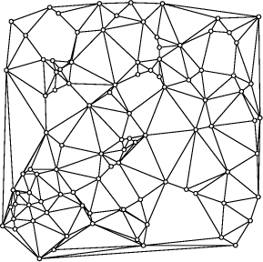
Figure 4: LMTskeleton for 100 points
that tends to yield some additional edges of LMT(S), indeed
exactly constructs LMT(S) provided the connectedness of this
structure.
The LMTskeleton clearly can be constructed in polynomial time, and
several variants have been considered in order to gain efficiency. A powerful
tool is preexclusion of edges before starting the LMTalgorithm, using
an exclusion region; see Das and Joseph [19]:
for an edge e, consider the two triangular regions with base e
and base angles  . If both regions contain points in S then e
cannot be part of MWT(S). If S is drawn from a uniform
distribution, reduction to an expected linear number of candidate edges
for MWT(S) is achieved, and nearlinear expectedtime implementations
of the LMTalgorithm exist. In fact, the LMTskeleton approach enables
the computation of a minimum weight triangulation for some 10 000 points
within half an hour. . If both regions contain points in S then e
cannot be part of MWT(S). If S is drawn from a uniform
distribution, reduction to an expected linear number of candidate edges
for MWT(S) is achieved, and nearlinear expectedtime implementations
of the LMTalgorithm exist. In fact, the LMTskeleton approach enables
the computation of a minimum weight triangulation for some 10 000 points
within half an hour.
Let us conclude with stating two open problems. The obvious one, of
course, is to theoretically resolve the complexity status of finding a
minimum weight triangulation. The second one could be intuitively stated
as follows: can we always find the same triangulation in two
different point sets? More precisely, can any two npoint sets
(that agree on the number of extreme points) be triangulated so as to give
isomorphic triangulations? No recent answers are available, except for
severe restrictions on either the shape of the point sets or on the number
of nonextreme points; see [5].
4 Subdividing a polygon in a natural way
Partitioning a complex geometric object into smaller and easier to deal
with parts is a first step in various algorithms in computational geometry.
As many planar geometric objects can be described sufficiently accuratly
by (straightline) polygons, partitioning algorithms for polygonal objects
have received particular attention.
Among the obvious (and for several situations sufficient) ways to subdivide
a (nonselfintersecting) polygon P is the partitioning into slabs
or into triangles. For example, P may be divided into parallel slabs
by cutting with vertical lines through its vertices. Or P may be triangulated,
by introducing diagonals between its vertices. In fact, triangulating an
nvertex polygon in O(n) time has been a tantalizing open
question which has not been settled till 1990; see Chazelle [17].
Obviously, a polygon P allows for many different slab partitions
or triangulations. Also, these structures will not reflect much of the
original shape of P, and thus cannot be called 'natural' partitions
of P in this sense. In numerous applications, like pattern recognition,
robotics, and GIS, a so/shy;called skeleton partition of P is
sought. Informally speaking, a subdivision into regions is meant which
reflects the geometric shape of P in an appropriate manner.
4.1 Medial axis and Voronoi diagram
The wellshy;known and widely used example of a polygon skeleton is the
medial axis of P, proposed by Preparata [33],
Kirkpatrick [30], and Lee [31].
This skeleton consists of all points inside the polygon which have more
than one closest point on the boundary of P. It is a treelike structure,
composed of straightline arcs and parabolically curved arcs, which partition
P into regions. Each region is the locus of all points closest to
a particular edge or vertex of P. The number of arcs remains linear
in the number n of vertices of P. The medial axis reflects
well the geometry of a polygon. The availability of relatively simple O(n
log n) construction algorithms3
makes it a suitable candidate for a skeleton description. However, it typically
contains curved arcs in the neighborhood of the polygon vertices. In comparison
to other polygon partitions, which are solely composed of straight line
segments, this yields disadvantages in the computer representation and
construction, and possibly also in the application, of this type of skeleton.
Before introducing an alternative skeleton structure which avoids this
shortcoming, let us briefly discuss the medial axis in the context of
Voronoi diagrams. Speaking sloppily, a Voronoi diagram is a partition
of a space U induced by a set S of objects that live in that
space. The scope of variations of Voronoi diagrams that have been investigated
within and outside computational geometry is vast;
3An O(n)
construction algorithm exists but lacks a simple implementation.
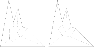
Figure 5: Angular bisector skeletons
see e.g. the survey papers by Aurenhammer and Klein [11,
10]. Still, they all fit into either framework of
definition below.
In the distance model, a distance function d is defined
that maps each element of S x U to a real number. The Voronoi
region of an object s S is the set of all elements  U
whose unique closest object with respect to d is s. The wavefront
model, on the other hand, prescribes for each object s S
a set of wavefronts that emanate from s and eventually cover the whole
space U. Wavefront propagation stops wherever two wavefronts collide.
The Voronoi region of an object s is the portion of U covered
by the wavefronts for s. In the classical case of a Voronoi diagram,
U is the Euclidean plane, S is a finite set of points, and
d is the Euclidean distance function. The wavefronts for each point
s S are circles centered at s. For the medial axis
of a polygon P, U is the interior of P, d is
the same as above, and S is the set of vertices and edges of P.
The distance model and the wavefront model are not equivalent, however.
The skeleton structure we are going to describe will have no interpretation
in the distance model. U
whose unique closest object with respect to d is s. The wavefront
model, on the other hand, prescribes for each object s S
a set of wavefronts that emanate from s and eventually cover the whole
space U. Wavefront propagation stops wherever two wavefronts collide.
The Voronoi region of an object s is the portion of U covered
by the wavefronts for s. In the classical case of a Voronoi diagram,
U is the Euclidean plane, S is a finite set of points, and
d is the Euclidean distance function. The wavefronts for each point
s S are circles centered at s. For the medial axis
of a polygon P, U is the interior of P, d is
the same as above, and S is the set of vertices and edges of P.
The distance model and the wavefront model are not equivalent, however.
The skeleton structure we are going to describe will have no interpretation
in the distance model.
4.2 Straight skeleton
In fact, the basic idea for obtaining a straightline skeleton
is neither complex nor new: use angular bisectors rather than 'distance'
bisectors for the polygon edges. However, extending angular bisectors until
they meet and continuing this way in an uncontrolled manner may result
in diffeerent and actually unintended structures; see Figure
5. Thereby, the number of skeleton arcs may grow beyond linear, and
even selfintersections (that is, no proper partitions) may arise. In fact,
and unlike the case of Voronoi diagrams, it is unclear how to come up with
a nonprocedural (and unique) definition of an angular bisector
skeleton. This fact might have kept off computational geometers from further
considering this concept.
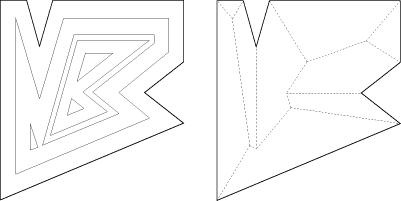
Figure 6: (a) Polygon hierarchy and (b) straight skeleton
A recent, and surprisingly simple, answer has been given in Aichholzer
et al. [3, 2]. The straight
skeleton, S(P), of a polygon P, is defined (via
the wavefront model) as follows. Shrink P, by continuously insetting
each of its vertices, so that at any particular time, every shrunken polygon
edge is parallel to the original, and the distance from the original is
the same for all shrunken edges. This makes each polygon vertex move along
the angular bisector of its incident edges, as long as the polygon boundary
does not change topologically. There are two possible types of changes:
(1) Edge event: An edge shrinks to zero, making its neighboring
edges adjacent now.
(2) Split event: An edge is split, i.e., a re ex vertex runs
into this edge, thus splitting the whole polygon. New adjacencies occur
between the split edge and each of the two edges incident to the reflex
vertex.
After either type of event, we are left with a new, or two new, polygons
which are shrunk recursively if they have nonzero area. The shrinking
process gives a hierarchy of nested polygons; see Figure
6(a). The straight skeleton, S(P), is defined as the
union of the pieces of angular bisectors traced out by polygon vertices
during this shrinking process. S(P) is a unique structure
defining a polygonal partition of P. Each edge e of P
sweeps out a certain area which corresponds to its region in S(P).
See Figure 6(b).
Compared to the medial axis of P, the straight skeleton
S(P) is also superior in the following respect. If
P is nonconvex, then S(P) is of smaller
combinatorial size. To be precise, if P is an ngon
with r reflex vertices then S(P) realizes
2n - 3 arcs whereas the medial axis of P realizes
2n + r 3 arcs, r of which are
parabolically curved. (For convex polygons, the two skeletons are identical.)
As a particularly nice property, S(P) partitions P
into polygons that are monotone in direction of their defining edge.
A drawback of S(P) is that it cannot be constructed
using the welldeveloped machinery for computing Voronoi
diagrams. The best known algorithm runs in roughly  time; see Eppstein and Erickson [23]. From the practical point of view, the
triangulationbased algorithm in [2]
simulating the wavefront movement is preferable in view of its almost
linear observed behavior. time; see Eppstein and Erickson [23]. From the practical point of view, the
triangulationbased algorithm in [2]
simulating the wavefront movement is preferable in view of its almost
linear observed behavior.
4.3 Applications
To demonstrate that S(P), beside its use as a skeleton
for P, is indeed a natural and useful subdivision, we briefly describe
some seemingly unrelated applications.
We first show that S(P) allows for a 3D interpretation
in a natural way. To this end, for a point  in the interior of P,
let T () denote the unique time when is reached by the first
wavefront edge. (The region of S(P) containing belongs
to the edge of P which sends out this wavefront edge.) Considered
as a function on the domain P, T () is continuous and piecewise
linear, that is, its graph in the interior of P,
let T () denote the unique time when is reached by the first
wavefront edge. (The region of S(P) containing belongs
to the edge of P which sends out this wavefront edge.) Considered
as a function on the domain P, T () is continuous and piecewise
linear, that is, its graph  is a polygonal surface in threespace.
The facets of project vertically to the regions of S(P).
Let us mention two applications where the construction of a surface from
a given polygon P comes in. is a polygonal surface in threespace.
The facets of project vertically to the regions of S(P).
Let us mention two applications where the construction of a surface from
a given polygon P comes in.
For example, P may be interpreted as an outline of a building's
groundwalls. The task is to construct a polygonal roof that rises over
P and whose roof facets are all of the same slope. For general shapes
of P, the construction of a 'roof', defined as a polygonal surface
with given facet slopes and given intersection with the ground walls, is
by no means trivial. In fact, roofs are highly ambigous objects; cf. Figure
5. The surface  obtained from S(P) constitutes
a canonical and general solution. Moreover, realizes exactly
2n - 3 arcs, the minimum for all possible roofs of an n-gon
P. Note that the medial axis of P is not at all suited as
a roof, as it would give rise to cylindrical roof facets. obtained from S(P) constitutes
a canonical and general solution. Moreover, realizes exactly
2n - 3 arcs, the minimum for all possible roofs of an n-gon
P. Note that the medial axis of P is not at all suited as
a roof, as it would give rise to cylindrical roof facets.
In this context, two generalizations of S(P) are appropriate.
First, the straight skeleton may as well be defined for general planar
straightline graphs G, not just for polygons. A 3D surface  can be
defined similarly as above. In addition, the concept of straight skeleton
is exible enough to be adapted to yield surfaces (and in particular, roofs)
with individual facet slopes. This is achieved by tuning the propagation
speed of the individual wavefront edges. Of course, this changes the geometric
and topological structure of the skeleton. can be
defined similarly as above. In addition, the concept of straight skeleton
is exible enough to be adapted to yield surfaces (and in particular, roofs)
with individual facet slopes. This is achieved by tuning the propagation
speed of the individual wavefront edges. Of course, this changes the geometric
and topological structure of the skeleton.
An interesting GIS application, which makes use of the general shape
of the underlying graph G, is the reconstruction of geographical
terrains. Assume we are given a map where rivers, lakes, and coasts are
delineated by polygonal lines, yielding a planar straight line graph G.
We are requested to reconstruct
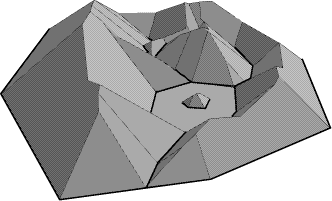
Figure 7: Terrain reconstructed from a river map
a corresponding polygonal terrain from G, possibly with additional
information concerning the elevation of lakes and rivers, and concerning
the slopes of the terrain according to different mineralogical types of
material. The surfaces resulting from S(G) and its modifications
seem to meet these general geographical requirements in an appropriate
manner. Figure 7 gives an example.
A related question is the study of rain water fall and its impact on
the oodings caused by rivers in a given geographical area. The amount of
water drained o by a river is usually estimated by means of the Voronoi
diagram of the river map. This models the assumption that each raindrop
runs o to the river closest to it, which might be unrealistic in certain
situations. The straight skeleton offers a more realistic model by bringing
the slopes of the terrain into play. In particular, the surface that
arises from S(G) has the following nice property: every raindrop
that hits a surface facet f runs o to the edge of G defining f.
Finally, an application of straight skeletons to origami design deserves
mention. A classical open question in origami mathematics is whether any
simple polygon P is the silhouette of (i.e., can be covered by)
a at origami. A recent and affirmative answer has been given in Demaine
et al. [20]. One of their approaches (the 'ring method')
uses the subdivision of P induced by a hierarchy of polygons that
arise during the shrinking process that yields S(P); cf.
Figure 6(a). It can be shown that each such polygonal
ring can be covered, and rings can be bridged appropriately, by a sequence
of paper folding operations. That is, the concept of straight skeletons
allows for a relatively simple proof of this classical origami conjecture.
References
1. O.Aichholzer, The path of a triangulation. Proc.
15 th Ann. ACM Symp. on Computational Geometry, 1999, 1423.
2. O.Aichholzer, F.Aurenhammer, Straight skeletons
for general polygonal gures in the plane. Proc. 2 nd Ann. Int. Computing
and Combinatorics Conf. CoCOON1996, Springer LNCS 1090, 117126.
3. O.Aichholzer, F.Aurenhammer, D.Alberts, B.G artner,
A novel type of skeleton for polygons. J. Universal Computer Science 1
(1995), 752761.
4. O.Aichholzer, F.Aurenhammer, R.Hainz, New results
on MWT subgraphs. Information Processing Letters 69 (1999), 215219.
5. O.Aichholzer, F.Aurenhammer, F.Hurtado, H.Krasser,
Towards compatible triangulations. 7 th Ann. Int. Computing and Combinatorics
Conf. CoCOON2001 (to be presented).
6. O.Aichholzer, F.Aurenhammer, G.Rote, M.Taschwer,
Triangulations intersect nicely. Proc. 11 th Ann. ACM Symp. on Computational
Geometry, 1995, 220229.
7. O.Aichholzer, F.Aurenhammer, H.Krasser, Enumerating
order types for small point sets with applications. 17 th Ann. ACM Symp.
on Computational Geometry, 2001 (to be presented).
8. O.Aichholzer, F.Hurtado, M.Noy, F.Santos, On the
number of triangulations every planar point set must have. Manuscript,
IGITU Graz, Austria, 2001 (submitted).
9. O.Aichholzer, H.Krasser, The point set order type
data base: a collection of applications and results. Manuscript, IGITU
Graz, Austria, 2001 (submitted).
10. F.Aurenhammer, Voronoi diagrams | a survey of
a fundamental geometric data structure. ACM Computing Surveys 23, 3 (1991),
345405.
11. F.Aurenhammer, R.Klein, Voronoi diagrams. In:
J.Sack, G.Urrutia (eds.), Hand book of Computational Geometry, Elsevier
Science Publishing, 2000, 201290.
12. F.Aurenhammer, Y.F.Xu, Optimal triangulations.
In: Encyclopedia of Optimization, Kluwer Academic Publishing, 2001 (to
appear).
13. P.Belleville, M.Keil, M.McAllister, J.Snoeyink,
On computing edges that are in all minimumweight triangulations. Proc.
12 th Ann. ACM Symp. on Computational Geometry, 1996, V7V8.
14. M.Bern, D.Eppstein, Mesh generation and optimal
triangulation. In: D.Z.Du, F.K.Hwang (eds.), Computing in Euclidean Geometry,
Lecture Notes Series in Computing 4, World Scienti c, Singapore, 1995,
47123.
15. A.Björner, M.Las Vergnas, B.Sturmfels,
N.White, G.Ziegler, Oriented Matroids. Cambridge University Press, 1993.
16. P.Bose, L.Devroye, W.Evans, Diamonds are not
a minimum weight triangulation's best friend. Proc. 8 th Canadian Conf.
on Computational Geometry, 1996, 6873.
17. B.Chazelle, Triangulating a simple polygon in
linear time. Discrete & Computa tional Geometry 6 (1991), 485524.
18. S.W.Cheng, Y.F.Xu, Constrained independence
system and triangulations of planar point sets. Proc. 1 st Ann. Int. Computing
and Combinatorics Conf. COCOON, Lecture Notes in Computer Science 959,
Springer Verlag, 1995, 4150.
19. G.Das, G.Joseph, Which triangulations approximate
the complete graph? Optimal Algorithms, Lecture Notes in Computer Science
401, Springer Verlag, 1989, 168 192.
20. E.D.Demaine, M.L.Demaine, J.S.B.Mitchell, Folding
at silhouettes and wrapping polyhedral packages: new results in computational
origami. Proc. 15 th Ann. ACM Symp. on Computational Geometry, 1999, 105114.
21. T.K.Dey, Improved bounds for planar ksets and
related problems. Discrete & Computational Geometry 19 (1998), 373382.
22. M.T.Dickerson, M.H.Montague, A (usually?) connected
subgraph of the minimum weight triangulation. Proc. 12 th Ann. ACM Symp.
on Computational Geometry, 1996, 204213.
23. D.Eppstein, J.Erickson, Raising roofs, crashing
cycles, and playing pool: Applications of a data structure for finding
pairwise interactions. Proc. 14 th Ann. ACM Symp. Computational Geometry,
1998, 5867.
24. S.Fortune, Voronoi Diagrams and Delaunay Triangulations.
In: D.Z.Du, F.K.Hwang (eds.), Computing in Euclidean Geometry, Lecture
Notes Series in Computing 4, World Scienti c, Singapore, 1995, 225265.
25. M.Garey, D.Johnson, Computers and Intractability.
A Guide to the Theory of NPcompleteness. W.H.Freeman (ed.), 1979.
26. J.E.Goodman, Pseudoline arrangements. In J.E.Goodman,
J.O'Rourke (eds.), Handbook of Discrete and Computational Geometry. CRC
Press LLC, Boca Raton, NY, 1997.
27. J.E.Goodman, R.Pollack, Multidimensional sorting.
SIAM J. Computing 12 (1983), 484507.
28. J.E.Goodman, R.Pollack, B.Sturmfels, Coordinate
representation of order types requires exponential storage. Proc. 21 st
Ann. ACM Sympos. Theory of Computing, 1989, 405410.
29. M.Keil, Computing a subgraph of the minimum
weight triangulation. Computational Geometry: Theory and Applications 4
(1994), 1326.
30. D.G.Kirkpatrick, Efficient computation of continuous
skeletons. Proc. 20 th Ann IEEE Symp. on Foundations of Computer Science,
1979, 1827.
31. D.T.Lee, Medial axis transform of a planar shape.
IEEE Trans. Pattern Analysis and Machine Intelligence PAMI4 (1982), 363369.
32. E.L.Lloyd, On triangulations of a set of points
in the plane. Proc. 18 th IEEE Symp. on Foundations of Computer Science,
1977, 228240.
33. F.P.Preparata, Steps into computational geometry.
Rep. R760, Coordinated Science Lab., Univ. of Illinois, Urbana, 1977,
2324.
34. M.I.Shamos, D.Hoey, Closest point problems.
Proc. 16 th IEEE Symp. on Foundations of Computer Science, 1975, 151162.
|