| Submission Procedure |
Perturbation Simulations of Rounding Errors in the Evaluation of Chebyshev SeriesRoberto Barrio Jean-Claude Berges Abstract: This paper presents some numerical simulations of rounding errors produced during evaluation of Chebyshev series. The simulations are based on perturbation theory and use recent software called AQUARELS. They give more precise results than the theoretical bounds (the difference is of some orders of magnitude). The paper concludes by confirming theoretical results on the increment of the error at the end of the interval [-1; 1] and the increased performance achieved by some modifications to Clenshaw's algorithm near those points. Key Words: Rounding errors, perturbation methods, Chebyshev polynomials, polynomial evaluation 1 IntroductionToday, numerical simulation is the most widely used method for evaluating physical systems. In order to obtain descriptive results of a physical phenomenon, a scientific software program must implement a mathematical representation of an actual problem using numerical resolution methods. To validate the simulation results, one has to evaluate the propagation of roundoff errors dependent on computer arithmetic units, as well as the impact of erroneous input data on the final result. This process guarantees that results can be trusted. Chebyshev polynomial series appear in several fields of scientific research and mathematics, as, for instance, in the resolution of partial differential equations by means of the Chebyshev collocation method [Canuto et al. 1988], in the approximation of functions [Schonfelder 1978] and in the compression of satellite ephemerides [Coffey et al. 1996]. Let pn(x) be one of such series with a finite number of terms, i.e.,
where Ti (x) are the Chebyshev polynomials of the first kind. A typical operation is the evaluation of (1) at one point x for which several algorithms have been proposed [Bakhvalov 1971, Clenshaw 1955, Forsythe 1957, Gentleman 1969]. Page 561 The numerical stability of those algorithms has been studied [Bakhvalov 1971, Oliver 1979], giving some theoretical bounds of the rounding errors. Following these studies Clenshaw's algorithm is recommended except for x near -1 and 1, where the Reinsch modifications to Clenshaw's algorithm [Gentleman 1969] are preferred. These theoretical bounds are very conservative, as they are of several orders of magnitude bigger than the real errors, and consequently, of limited use in practical situations. For this reason, we chose to study ``realistic'' rounding errors for some Chebyshev series by using each of the proposed algorithms in turn in order to confirm the theoretical analysis (for more details see [Barrio and Berges 1997]). These analyses are of practical interest due to the need to choose one or several algorithms for accurate evaluation of any specific series. 2 Perturbation analysisWe thus used modern software called AQUARELS [Berges 1995, Erhel et al. 1991, Francois 1989] to do perturbation analysis in order to obtain estimations of the rounding errors. This program provides a problem solving environment for controlling and improving the numerical quality of scientific software. The simulation is based on random perturbations of the last bit of the result in each elementary operation. This kind of methods has proven its usefulness in scientific computing [Chesneaux 1994]. The algorithms analyzed are those of: Forsythe, Clenshaw, and Bakhvalov and also the Reinsch modifications near x = -1 (Reinsch(-1)) and near x = 1 (Reinsch(-1)). In the tests, four kinds of Chebyshev series were used; the first (P1) with 6000 random coefficients normally distributed with mean 0 and variance 1, the second (P2) with monotonically decreasing coefficients, ci = 1=i2 (i = 1,..., 6000), and the third (P3) and the fourth (P4) consisted of the 3000 first coefficients of the development of two functions in Chebyshev polynomials:
2.1 Theoretical boundsThe theoretical bounds [Bakhvalov 1971, Oliver 1979] of the rounding errors are usually given up to the first order on the unit roundoff (u) of the computer used, i. e.,
where Figure 1 shows the theoretical error bounds (factor k). The left-hand
side shows the bounds for x Page 562 function. Also, it may be observed that, a priori, Reinsch's
algorithm adapted for values near x = -1 works better in that interval,
while the performance is worse near x = 1. Something similar occurs
with the other algorithm of Reinsch for the case x = 1. At these
values ( Taking into account the figures of the theoretical error bounds leads
to the same recommendations as Oliver, i. e. using the algorithm of Reinsch(-1)
for x
Figure 1: Theoretical error bounds. Page 563 2.2 Numerical testsThe previous sub-section dealt with the theoretical bounds, but the question remains as to what happens in a real problem? How accurate are the theoretical bounds? In some algorithms the theoretical bounds are quite accurate and yield good estimations of the rounding errors, but in others there are some ``pathological'' problems with a bound of several orders of magnitude bigger than average. Therefore, in such algorithms the theoretical bound would be of little use because it accounts for the worst-case propagation of errors. Due to the big size of the theoretical bounds of some algorithms, specially near x = -1 and x = 1, it appeared to be worthwhile to do some numerical analysis. As mentioned above, Aquarels software with double precision was used. AQUARELS applies a perturbation method in order to estimate ``realistic'' error bounds for some problems of interest. For each evaluation algorithm, each series, and each point of evaluation
x Table 1: Results of the normality test of Shapiro and Wilk. The significance
level is
Let xi
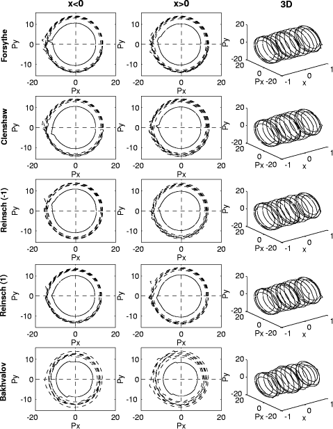
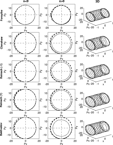
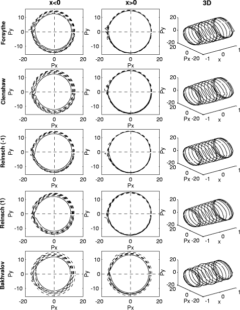
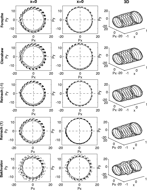
In order to represent all the perturbation tests we used what we have called the logarithmic polar representation. In 2D, this representation of the absolute Page 564 rounding errors consists of representing on the plane
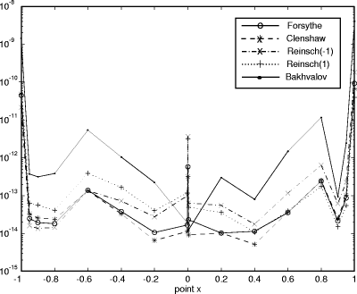
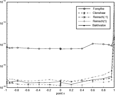
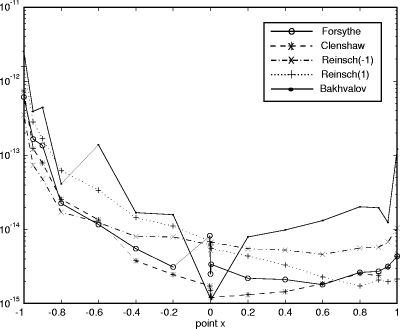
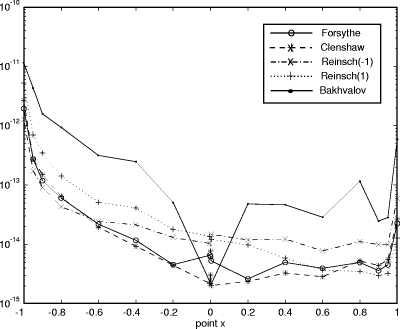
For the relative rounding errors we used Figures 2, 3, 4 and 5 show the logarithmic polar representation of the simulation errors and Figures 6, 7, 8 and 9 show the standard deviation, in a logarithmic scale. The increment at the ends of the interval appears in every algorithm and problem, but without the symmetry of the theoretical bounds. In each problem (except P2) the worst performance is presented for the Bakhvalov algorithm. For the P1 problem the behavior of the algorithms is quite similar, except for the Bakhvalov one. In general, the best performance was achieved using the Clenshaw algorithm, but near the ends, a slight improvement was found for the Reinsch algorithms. For P2 the Forsythe algorithm worked ``badly'', due to the particular behavior of the coefficients, monotonically decreasing in size. Thus, it is better to begin the evaluation from the last coefficients (the Forsythe algorithm is the only one that begins from the first ones). The ``good'' behavior of this analysis is shown in 2D in the joined curves and in 3D in the almost cylindrical figure. On P3 and P4 we observed that the rounding errors increase with the complexity of the function to be approximated. It has been demonstrated that the theoretical bounds are some orders of magnitude higher than the simulations. Besides, for the Bakhvalov algorithm these bounds are of little use, due to the unknown coefficient in the theoretical bound. Therefore, our recommendations on the choice of one algorithm, taking into account only the rounding errors, are similar to those resulting from the theoretical analysis, i. e.: in general, the Clenshaw algorithm should be used and near the ends the Reinsch algorithms. Table 2 shows the ``best'' algorithm depending on the interval of the variable x. Table 2: ``Recommended'' algorithms.
Page 565 3 ConclusionsThe numerical tests confirmed the theoretical results on the increment of the error at the ends of the interval [-1; 1] and the better performance of some modifications of the Clenshaw algorithm at those points. It should be pointed out that, as the differences on the rounding errors observed in the simulations for the different algorithms are in general very small, it is not worth using other algorithms than that of Clenshaw due to its good performance in the tests and its cheaper evaluation cost. It may be concluded that it is worthwhile controlling rounding errors via perturbation analysis as a complement to theoretical studies of the error bounds since this control serves as a numerical validation and analysis of the theoretical bounds. Also, it can be useful in a preliminary study of the stability of new algorithms, when no bounds are known or when the determination of bounds is a difficult task. 4 AcknowledgmentsThe first author has received partial support from both the Département de Mathématiques Spatiales at the Centre National d'Etudes Spatiales (Toulouse, France) and from project PB95-0807 of the Ministerio de Educacióon y Ciencia (Spain). References[Bakhvalov 1971] Bakhvalov, N. S: ``The stable calculation of polynomial values''; J. Comp. Math. and Math. Phys., 11 (1971), 1568-1574. [Barrio and Berges 1997] Barrio, R. and Berges, J. C.: ``Analysis of Rounding Errors in the Evaluation of Chebyshev Series''; CNES Report DGA/T/TI/MS/MN 97- 222, Toulouse, France (1997). [Berges 1995] Berges, J. C.: ``Improvement of the accuracy of Space Dynamics Software: The Toolbox AQUARELS''; proc. SCAN'95 (1995). [Canuto et al. 1988] Canuto, C., Quarteroni, A., Hussaini, M.Y. and Zang, T.: ``Spectral Methods in Fluid Mechanics''; Ed. Springer-Verlag, New York (1988). [Chesneaux 1994] Chesneaux, J. M.: ``The equality relations in scientific computing''; Numerical Algorithms, 7 (1994), 129-143. [Clenshaw 1955] Clenshaw, C. W.: ``A note on the summation of Chebyshev series''; MTAC, 9 (1955), 118-120. [Coffey et al. 1996] Coffey, S., Kelm, B. and B. Eckstein: ``Compression of Satellite Orbits''; AAS 96-125 (1996). [Cox 1993] Cox, M.G.: ``Reliable determination of interpolating polynomials'', Numerical Algorithms, 5 (1993), 113-154. [Erhel et al. 1991] Erhel, J. and Philippe, B.: ``Design of a toolbox to control arithmetic reliability''; proc. SCAN'91 (1991). [Forsythe 1957] Forsythe, G. E.: ``Generation and use of orthogonal polynomials for data fitting with a digital computer''; J. SIAM, 5 (1957), 74-88. [Francois 1989] Francois, P.: ``Contribution à l'étude de méthodes de contrôle automatique de l'erreur d'arroundi: la methodologie SCALP''; Ph.D. Dissertation (in French), University of Grenoble, France (1989). Page 566 [Gentleman 1969] Gentleman, W. M.: ``An error analysis of Goertzel's (Watt's) method for computing Fourier coefficients''; Comput. J., 12 (1969), 160-165. [NAG 1993] NAG: ``NAG Fortran Library Manual, Mark 16''; Volume 1 (1993). [Oliver 1979] Oliver, J.: ``Rounding error propagation in polynomial evaluation schemes''; Journal of Computation and Applied Mathematics, 5 (1979), 85-97. [Royston 1982] Royston, J. P.: ``An extension of Shapiro and Wilk's W test for normality to large samples''; Appl. Statist., 31 (1982), 115-124. [Schonfelder 1978] Schonfelder, J. L.: ``Chebyshev expansions for the error and related functions''; Maths. Comput., 32 (1978), 1232-1240. Page 567
Figure 2: Logarithmic polar representation of the error for the problem P1. Page 568
Figure 3: Logarithmic polar representation of the error for the problem P2. Page 569
Figure 4: Logarithmic polar representation of the error for the problem P3. Page 570
Figure 5: Logarithmic polar representation of the error for the problem P4. Page 571
Figure 6: Standard deviation of the rounding errors in the P1 problem.
Figure 7: Standard deviation of the rounding errors in the P2 problem. Page 572
Figure 8: Standard deviation of the rounding errors in the P3 problem.
Figure 9: Standard deviation of the rounding errors in the P4 problem. Page 573 |
|||||||||||||||||||||||||||||||||||||||||||||||||||||||||||||||||||||||||||||||||||||||||||||||||||||||||||||||||
 ci Ti (x), with
x
ci Ti (x), with
x  [-1; 1];

 (x) is the calculated value of pn (x).
  , 1 -
, 1 -  -1;
-1; 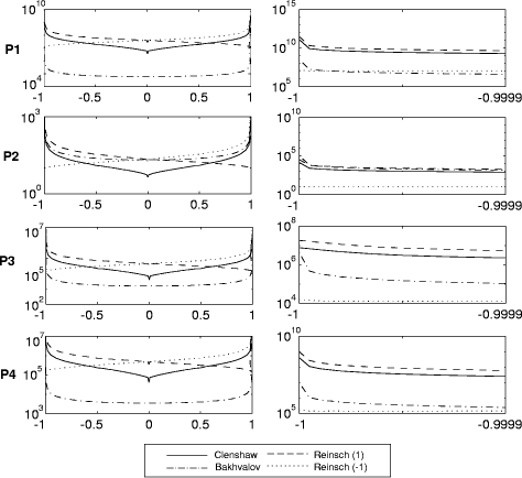
 = 0.05. The values of the statistic W of the simulations are bigger
than the corresponding tabulated values of W for = 0.05 and N =
100 (the p-value
= 0.05. The values of the statistic W of the simulations are bigger
than the corresponding tabulated values of W for = 0.05 and N =
100 (the p-value 
 j
j 
 instead of
  . In 3D, the representation
is similar, but with x as the third coordinate. Moreover, the data rij
was sorted from bigger to smaller
. In 3D, the representation
is similar, but with x as the third coordinate. Moreover, the data rij
was sorted from bigger to smaller  in order to smooth the curve. Also, with
the re-ordering, the negative errors are plotted on the lower part of the
graph, while the positive are on the upper part. These representations
of the rounding errors enabled us to better visualize their behavior.
in order to smooth the curve. Also, with
the re-ordering, the negative errors are plotted on the lower part of the
graph, while the positive are on the upper part. These representations
of the rounding errors enabled us to better visualize their behavior.